Comparative compositions of Pluto and friends, even long-distant friends.

Reposted from https://blogs.nasa.gov/mission-ames/2013/07/23/comparative-compositions-of-pluto-and-friends-even-long-distant-friends/.

Continuing coverage of the July 22, 2013 first day of the Pluto Science Conference being held this week in Laurel, MD.

Bill McKinnon (Washington University) next provided an engaging talk about implications for composition and structure for Pluto and Charon.

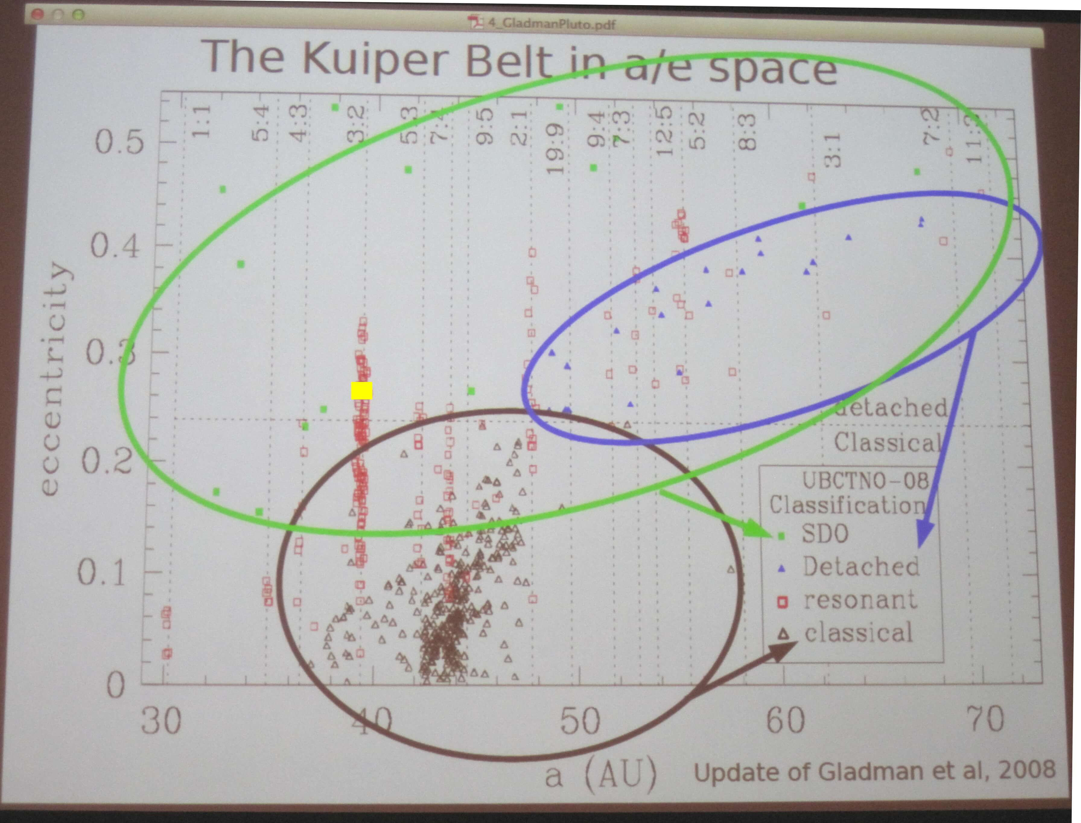
Where did Pluto Accrete (i.e. where was Pluto born)? Pluto is not alone in its location on that a/e plot for Trans-Neptunian Objects (see previous posting).  It’s part of an ensemble of bodies on the 2:3 resonance with Neptune, coined the group “Plutinos.” Was Pluto formed around 33 AU (Malhotra 1993, 1995) and then migrated outward? What does this Nice I Model (Levinson et al 2008) which migrates the giant planets predict for the KBO population? The Nice I Model implies that for Pluto, Pluto could have formed 20-29 AU (i.e. closer in) to allow it to achieve its high inclination. Then a subsequent model, Nice II (Levinson et al 2011), suggests Pluto may have formed in the 15-34 AU range. This is in okay-agreement with accretion models since Pluto, a 1000-km size body, would need 5-10 million years (i.e. within a nebular life) if it were formed in the 20-25 AU range. McKinnon’s best guess: Pluto formed between 15-30 AU.

How long did accretion take and what are the implications (i.e. how long for Pluto to grow up)? If we have an accretion time (10’s of million years), there is time enough to form Aluminum-26, which provides a form of heat through its decay. Heat then can melt ices and create a differentiated body (i.e., rocky core, icy mantle) and also drive water out. McKinnon’s best guess: Pluto formed rapidly and early.

What are Pluto & Charon made of? They are understood to be made of rock+metal, volatile ices, and organics, with rock+metal more than ice, and ice more than organics. The rock will be some combination of hydrated & anhydrous silicates, sulfides, oxides, carbonates, chondrules, CAIs (calcium-aluminum-rich inclusions), CHONPS (carbon, hydrogen, nitrogen, oxygen, phosphorus, and sulfur). We don’t really know what sort of composition these KBO volatile ices: will they be more like Jupiter Family Comets or Oort Comets? And we know even less about organic components: will the Nitrogen to Carbon ratio tell us whether KBO N2 (nitrogen) comes from organics rather than NH3 (ammonia)? Solar models (which lock up CO (carbon-monoxide) into carbon) can influence understanding of what rocks in the outer solar system are made of but their models are not in agreement with the best understanding of Pluto/Charon make-up. McKinnon’s best guess: Rock/Ice nature of Pluto-Charon is 70/30.

What are the implications for Pluto & Charon internal structure? New Horizons will not directly detect the differentiation state of Pluto & Charon because it does not fly close enough.

Alain Doressoundiram (Paris, France) came next. Using MIOSTYS, multi-fiber front-end to a fast EMCCD camera, on a 193 cm telescope in France, they observe outer solar system bodies using stellar occultations. Other science objectives for variable stars, transiting exoplanets. They confirmed two TNO occultation events, one in 2009 and one in 2012 and continue monitoring.

Luke Burkhart (Johns Hopkins University) talked about his work on a “Non-linear satellite search around Haumea.” Haumea is another Trans-Neptunian Object (TNO) that has multiple satellite companion, like Pluto. Using HST (10 orbits) they observed the Haumea system and used a method of stacking & shifting to identify satellites. But this method fails to capture objects which are close in, moving fast, and on highly curved orbits. So they developed a new method using a non-linear shift-rate. Their approach, when applied to the Haumea system, had a null-result. However, this approach could be used on images of the Pluto system and other TNOs.  Specifically, in answer to a question from the audience, Luke would be eager to use his technique on any of those long-range KBO targets the New Horizons project is currently investigating.

eighttnos

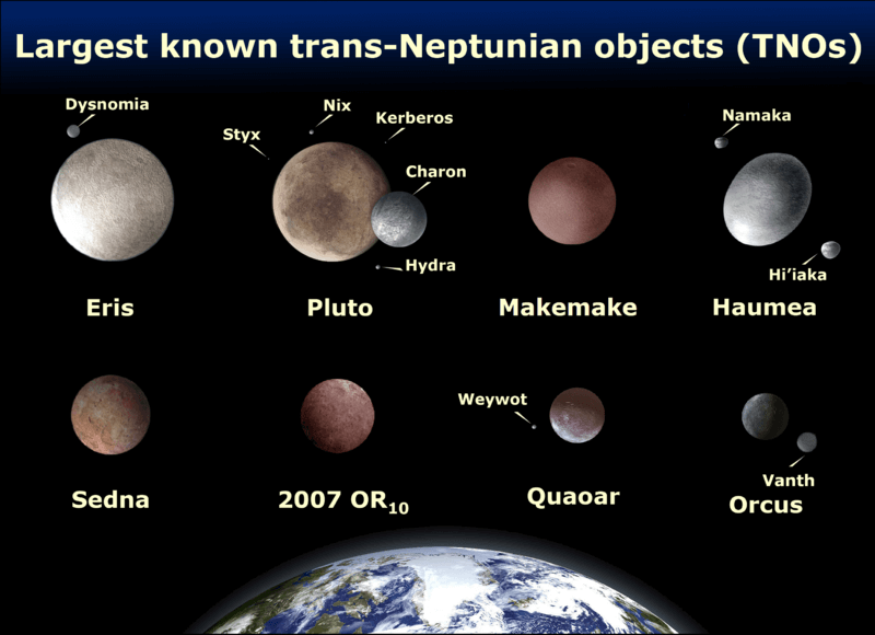
Family portraits of the eight largest trans-Neptunian objects (TNOs) (From http://en.wikipedia.org/wiki/Trans-Neptunian_object). Pluto is shown with its 5 companions.

Andy Rivkin (JHU/APL) ended the afternoon’s lively discussion by addressingDistant Cousins: What the Asteroids Can Teach us About the Pluto System”. He started his talk with a comparison of sizes between Ceres (the largest asteroid in the asteroid belt between Mars and Jupiter) and the Pluto System. He used as his framework Emily Lakdawalla’s chart, which can be found on the Planetary Society blog http://www.planetary.org/multimedia/space-images/charts/relative-sizes-pluto-system.html.

Here the relative sizes of objects in the Pluto system are represented by objects from the Saturn system. Saturn’s moon Rhea serves as Pluto, Dione as Charon, Prometheus as Nix, Pandora as Hydra, Helene as Kerberos, and Telesto as Styx. Superimposed is where Ceres (an asteroid in our asteroid belt between Jupiter & Mars) fits on this scale. Andy Rivkin did a comparison of his observations of Ceres to postulate what that might mean for the Pluto system.

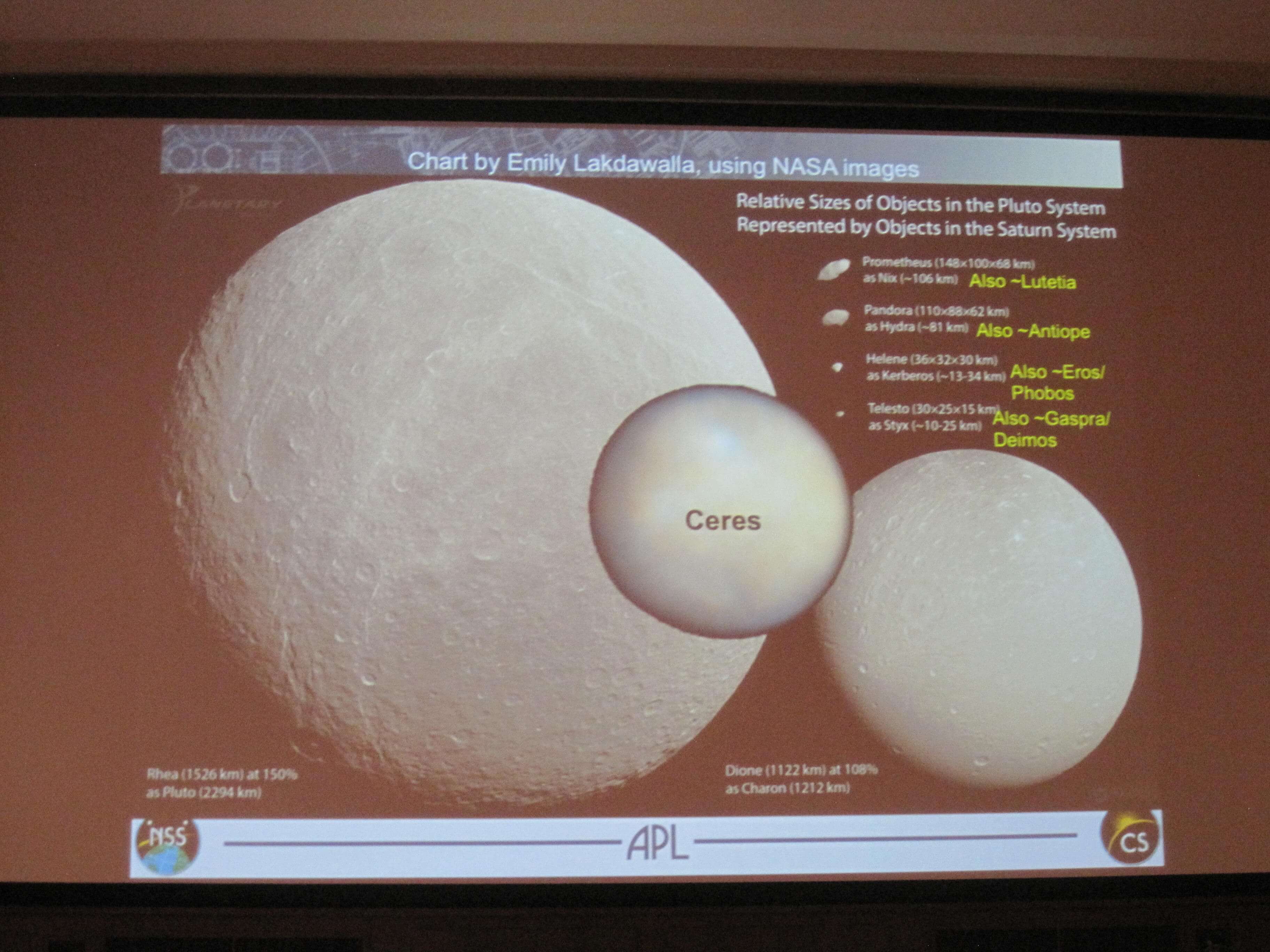
Pluto system and Ceres shown to scale, represented by objects from the Saturn system.

Ceres has an icy interior, but much too warm to keep ice on surface. HST images reveals rather smooth surface. IR spectra (from reflected sunlight) are very rich and indicative of ice-type features. Could there some sort of layering? On Pluto, you could have the same thing, but it’s also cold enough for ice to remain on the surface. There is also a mystery that several large C asteroids have similar 3 micron spectra to Ceres like 10 Hygiea and 704 Interamnia.

Implications for Pluto: Large main-belt asteroids could serve as comparisons for KBOs. Geophysical comparisons may be easier than compositional ones.

So the big take-away from the introductory talks on the “Kuiper Belt Context” is that we can learn more by sharing the knowledge: Learning from Other Bodies  (Other TNOs, Comets, Asteroids) will help us learn more about Pluto & Charon, and vice versa.

Finding that distant KBO needle in a deep space haystack.

Reposted from https://blogs.nasa.gov/mission-ames/2013/07/23/finding-that-distant-kbo-needle-in-a-deep-space-haystack/.

Next up at the Pluto Science Conference were a series of talks dedicated to recent work in the searches for another Kuiper Belt Object (KBO) for the New Horizons spacecraft to fly by after its Pluto fly-by. Fuel on board the New Horizons spacecraft after the July 2015 Pluto fly-by could enable a fly-by of a distant KBO in the late 2010s through 2020s, pending identification of targets reachable within New Horizon’s remaining fuel budget.

John Spencer (SwRI) has been leading the ground based campaign to search for New Horizons’ next target. With an on board ~0.13 km/s delta-v (measure of propellant), traveling at 14 km/s, this translated to a ~0.5 deg half-angle cone through the Kuiper Belt for accessible targets, a type of “survey beam.” Previous KBO searches had been for R>26.0 over 1-2 degrees. But right now Pluto is in Sagittarius which is in the direction of the Galactic Center and there are a lot of other stars in the field that make searching for a slowly-moving object, this KBO, difficult.

img_1135

Above are what the star fields the team is inspecting look like. They observe the same star field night after night and look for shifts in a object between frames, indicating it’s a KBO and not one of the “fixed stars.”

611px-outersolarsystem_objectpositions_labels_comp

“Known objects in the Kuiper belt, derived from data from the Minor Planet Center. The pronounced gap at the bottom is due to difficulties in detection against the background of the plane of the Milky Way.” This is exactly where John Spencer and his team are focusing their efforts because a subsection of that part of the sky is what is reachable by the New Horizons spacecraft after 2015. Image taken from http://en.wikipedia.org/wiki/Kuiper_belt.

The ground based search program area is entering a sweet spot, where they can cover a smaller area of sky from the Earth that falls within the expected New Horizons travel zone.

The team has found 31 objects from 2011 data including a TNO. However, as of 2012 season, they have not found an object that could have a fly-by encounter by the New Horizons spacecraft.  But there are three objects (2011 JW31, 2011 JY31, 2011 HZ102) that New Horizons could get to within 0.15-0.2 AU of in 2018-2019. The team is in the middle of the 2013 observing season and based on the current number densities they are predicting to see 1.78 objects down to  R=26.0mag and 4.15 objects in 26.5 mag.

Alex Parker (one more month at Harvard before moving to Berkeley) provided a more in depth view of unique observations New Horizons can still make of these long-distance KBO fly-by, that is, a fly-by in the 0.1-0.2 AU range of the spacecraft. At 0.2 AU range, New Horizons’ LORRI will have 140 km/pixel range compared to our “sharpest eyes” by Hubble at 1200 km /pixel from low-Earth orbit.

His excitement over the unique discovery space New Horizons provides that you cannot get from anywhere else: Proximity. High angular resolution. High phase angles.

He’s been studying trans-Neptunian binaries as binaries provide a direct mechanism to measure their masses. “Wide” Kuiper Belt binaries have been discovered already (e.g.  Gemini observations of wide binaries 2006 BR284 separated by 0.82 arcseconds; 2000 CF105 separated by 0.95 arcseconds).

To visualize a ride on looking over the New Horizons shoulders as it journeys into the Kuiper belt, check out this one of Alex Parker’s visualizations at Vimeo.com/alexhp/newhorizons.

Make note to hold onto your seat when the craft enters the Cold Kuiper Belt region in 2018!

Susan Benecchi (Carnegie Institute) rounded out the talks with HST Follow-Up Observations of Long-Range Candidates for New Horizons post Pluto. They observed 2011 JW31, 2011 JY31, and 2011 HZ102 with HST. Those objects had been detected with the KBO ground based search program described by John Spencer and Alex Parker (previous presentations). Her team has not confirmed detection of 2011 JW31. Her team has confirmed the colors of the two other objects being “red” which is consistent with the Cold Classical Population (i.e. primordial). Implications for New Horizons: HST can provide this extra characterization step for new candidates.

Gustavo Beneditti-Rossi (Brazil) described a summary of “Astrometric Analysis of 15 years of Pluto Observations.” Using the Pico dos Dias Observatory (1.6m and 0.6m telescopes), they monitored Pluto-Charon (which is not separated in their data) for 154 nights over 1995 to 2012. They do refraction correction (due to viewing angle from earth) and photo-center correction (due to the fact they cannot separate Pluto from Charon). And show that their tracking of Pluto’s location is in agreement with occultation data.

To end this post, I could not resist showing you Alex Parker’s vision of what New Horizons brings to this field of study. He created this montage of images illustrating the proximity (within artistic license) and equally important the high phase (objects as crescents) and high angular resolution (we can see surface features), all that New Horizons will provide in 2015 that no other observation platform can.

parker_nh_montage

2015 will be the “Year of Pluto” and so much more!

Pluto, “King of the Kuiper Belt, Prince of the Plutinos.” Certainly an object that inspires odes, songs, and ballads.

Reposted from https://blogs.nasa.gov/mission-ames/2013/07/23/pluto-king-of-the-kuiper-belt-prince-of-the-plutinos-certainly-an-object-that-inspires-odes-songs-and-ballads/.

After the New Horizons’ instrument overviews on the first day at the Pluto Science Conference (Jul 22, 2013, we jumped right into Pluto in the Kuiper Belt Context.

Brett Gladman (University of British Columbia, Vancouver, Canada) started the conversation by addressing “How does Pluto fit in our understanding of the Kuiper Belt?”

But before we get into that, discussing the Kuiper belt today can be pretty complex. It was only discovered in 1992, but in the years since, over 130,000 bodies with sizes 100 km and larger have been identified (Petit et al 2011), with Pluto being the largest member.

So when we start looking at large numbers of objects, it’s time to classify. So a typical plot to describe these “populations” is shown below, where semi-major axis (distance of body from the Sun) is plotted (horizontal axis, labeled ‘a’ in units AU, where 1 AU is the distance of the Earth from the Sun, Jupiter is ~5 AU, Saturn ~10AU) versus eccentricity (value between 0 and 1 that describes how circular an orbit it, e=0 is circle, e=1 is parabola, 0<e<1 describes ovals).

And then you have your Classical, your Cold Classical, Hot Classical, Detached, Resonant, and SDO (aka Scattered Disk Objects), etc. Sometimes they group together, others are more uniform across the parameter space.

Kuiper Belt in “a/e space.” Cold classical (black open triangles). Resonant Kuiper (open red square). Detached (blue triangles). Pluto is indicated with the yellow-box, it’s a Resonant, as it is in 3:2 Resonance with Neptune. This group of objects, all in 3:2 Resonance with Neptune are the “Plutinos.” (that clumping around 40 AU, red triangles, spanning over a range of e). Resonance numbers are shown at the top of the graph.

Plutinos are also a family of TNOs, Trans-Neptunian Objects, characterized by being in 3:2 mean-motion resonance with Neptune (i.e., every time Neptune makes 3 trips about the Sun, the Plutinos make 2 trips). Plutinos are the most dominant of the TNOs. Less numerous are the 1:1 objects, objects known as Trojans.

Definitely KBO soup!

For more information about TNOs and their period relationships with Neptune https://en.wikipedia.org/wiki/Resonant_trans-Neptunian_object.

After getting down those nomenclature basics, Brett Gladman (who is also lead for a huge ground-based survey of KBOs called the Canada-France Ecliptic Plane Survey/CFEPS) discussed the strengths and pitfalls of the theories put forward to explain the formation and structure of this complex KBO menagerie.

For more information about CFEPS check out http://www.cfeps.net/.

How did Pluto get to where it is today? Two leading theories (1) Resonant sweeping of objects formed in TNO regions and (2) resonant trapping explain many things, but no published models explain those resonant structures of the Kuiper belt. And any of these models have issues with the classical and scattering disk populations as well. Theorists, better sharpen your pencils.

So he left us with questions to ponder. Is there a cold primordial Kuiper Belt with edge at 45 AU? Did Pluto likely form as one of hundreds to thousands of >1000km embryos? Did some of these become implanted into the nearby non-scattering belt? Are there others out beyond 100 AU (considered likely, but to discover them, you need to get down to 23-24th mag which is beyond the current survey capabilities until new telescopes and.or techniques come available)?

No doubt, searches for more TNOs will continue, the classification of the KB will undergo evolution, and theorists will refine their models. And New Horizons will provide a unique data set of an up-close-and-personal visit to Pluto and its companions to help constrain those models.

800px-thetransneptunians_73au-svg

Putting Centaurs and TNOs in Context. This time plotting inclination (the degrees from the ecliptic plane) vs. semi-major axis in AU. Object sizes are reflected in the symbol sizes. Location of Saturn, Uranus and Neptune are shown. Just another way to look at that awesome & diverse Outer Solar System. From: https://en.wikipedia.org/wiki/Trans-Neptunian_object.

Next, Cesar Fuentes (Arizona State) phoned in about his work on the “Size Distribution (SD) of the Kuiper Belt.” Size distribution is basically counting the number of objects as a function of size.  Coagulation (of small particles) and gravitation instability (of larger particles) shape the size distribution. Size distribution is expected to change due to collisions. Different distances from the sun also appear to have different size distributions.

He stepped us through recent size distribution models from Schlichting, Fuentes & Trilling (2013) and Kenyon & Bromley (2013) where they even have some including the “collisional factor” influence on the size distribution over time periods.

All the Size Distributions show a “rollover” around H~9, D=70km. Nesvorny et al. 2013 investigates this further. Is the break due to collisional and therefore separate the primordial from the evolved KBO populations?

Even more questions to ponder:  Can we use size distributions to evaluate primordial from the evolved KBO populations?

And then he left us with a tantalizing experiment with the New Horizons mission: If New Horizons can provide data sets enabling “crater counting,” we will be able to measure the impactors on Pluto. This can aid in understanding KBO populations, addressing specifically, formation time, timescales for surface activity, and origins of bodies like Nix & Hydra. What would a 0.1-100 km impactor size distribution look like?

Pluto, be it Prince of the Plutinos or King of the Kuiper Belt, will always remain a key part to these questions above. And data sets from New Horizons will provide many new angles to answering questions about “Where did Pluto form and why did it wind up where it is now.”

Introducing the New Horizons Instrument Menagerie

Reposted from https://blogs.nasa.gov/mission-ames/2013/07/23/introducing-the-new-horizons-instrument-menagerie/.

During the first day of the Pluto Science Conference, being held July 22-26, 2013, in Laurel, MD, the conference participants listened to a series of talks describing the rich instrument suite aboard the New Horizons Spacecraft. This entry is just a very brief synopsis of the instruments.

Ralph, Alice, MVIC, LEISA, LORRI, REX, SWAP, PEPSSI, SDC. Those are instrument names and acronyms of the New Horizons science instruments.

nh_instrument_suite
New Horizons Instrument Suite at a Glance

LORRI (Long Range Reconnaissance Imager), among many things, “Enables Far-Out Encounter Science. ” That is, at 10 weeks from closest approach, LORRI can observe the Pluto system with spatial resolution better than Hubble. It is a visible camera, equipped with a 1024 x 1024 pixel CCD, with a 0.29 x 0.29 degree field of view (5 microradian pixel iFOV). LORRI also will be used, on approach, for optical navigation. The LORRI Instrument Principal Investigator and Instrument Scientist is Andy Cheng (JHU/APL) and Hal Weaver (JHU/APL), respectively.

Ralph & Alice form New Horizons’  “Remote Science Suite.” Ralph is both a color-imager (MVIC) and an infrared mapping spectrometer (LEISA). Alice is a ultraviolet spectrometer.

Ralph’s MVIC (Multi-Spectral Visible Imaging Camera) consists of seven independent CCD arrays. Four channels are filtered to map blue (400-550 nm), red (540-700 nm), near infrared (780-975 nm) and a narrow methane absorption band (860-910 nm). Six of the MVIC arrays (including all the filter channels) have a 5.7 x 0.037 degree field of view (20 microradian pixel iFOV). LEISA (Linear Etalon Imaging Spectral Array) is a grating spectrometer covering 1.25 to 2.5 microns wavelength range at a resolving power of R~240. A second segment covers 2.1 to 2.25 micron range with a resolving power of R~560. The Ralph Instrument Principal Investigator and Instrument Scientist is Alan Stern (SwRI) and Dennis Reuter (NASA Goddard), respectively.

Alice is an ultraviolet imaging spectrometer. It has two entrance apertures, a large airglow channel and a small SOCC aperture for solar occultation measurements. The entrance slit has two sections, a “box” with a 2.0 x 2.0 degree field of view, and a “stem” with a 0.1 x 4.0 degree field of view. The wavelength coverage spans from 520 to 1870 Angstroms, with a resolution of 3.6 Angstroms.  The Alice Instrument Principal Investigator and Instrument Scientist is Alan Stern (SwRI) and Maarten Versteeg (SwRI, San Antonio), respectively.

REX, New Horizons’ Radio Science Experiment, is enabled by adding a small amount of signal processing hardware to the existing communication hardware on New Horizons’ main antenna. It will be used, among other observations of Pluto, to showcase a “Different Kind of Radioscience” via 20kW uplink experiments from the DSN during the Pluto and Charon occulations at flyby. The REX Principal Investigator and Instrument Scientist are G.L. Tyler and Ivan Linscott (Stanford University), respectively.

PEPSSI (Pluto Energetic Particle Spectrometer Science Investigation) & SWAP (Solar Wind Around Pluto) are modern particle instruments designed to capture Pluto’s interaction with the solar wind. PEPSSI can measure ions and electrons from 10s of keV to 1 MeV over a 160 x 12 degree fan-shapped beam. SWAP can measure particles with energies 35 eV to 7.5 keV over a 276 x 10 degree field of view. PEPSSI’s Principal Investigator and Instrument Scientist are Ralph McNutt (JHU/APL) and Matthew Hill (JHU/APL). SWAP’s Principal Investigator and Instrument Scientist are David McComas (SwRI, San Antonio) and Heather Elliott (SwRI, San Antonio).

SDC, the Student Dust Counter, designed and built by students at the University of Colorado, Boulder, is “The First Student Experiment on a Deep-Space Probe.” The Principal Investigator is Mihaly Horanyi (University of Colorado). There have been numerous Instrument Scientists, all students at Univ. of Colorado. The current Instrument Scientist is Jamey Szalay. Students continue to be active in supporting data analysis as SDC collects dust rates on its voyage through the solar system. More information about the SDC and the students behind it at http://lasp.colorado.edu/sdc/.

More details about each of the instrument descriptions and performance can be found at http://pluto.jhuapl.edu/Mission/Spacecraft/Payload.php.

ast-new-horizons-instrument-outline
Locations of the science instruments on the New Horizons Spacecraft


The Architecture of New Horizons’ Pluto Fly-By Sequence

Reposted from https://blogs.nasa.gov/mission-ames/2013/07/22/the-architecture-of-the-pluto-fly-by-sequence/.

In her presentation at the Pluto Science Conference, Dr. Leslie Young (SwRI), deputy Project Scientist and chief architect of the Pluto Encounter Sequence, stepped us through the New Horizons’ Science Objectives and the types of observations that will be pre-programmed aboard the craft for the entire year of 2015. Unique science is not just around Pluto Closest Approach on Tues, Jul 14, 2015, but many months prior and post the encounter. Although most of the “Group 1” (see below for description) science objectives for the mission will be met by measurements made in the -2hr to +3hr from closest approach. Closest approach is on July 14, 2015.

leslie_young_group_objectives
Leslie Young (deputy Project Scientist) describes the overview of the science highlights for the year 2015. Also shown in the slide is a mapping of the Science Objectives per each phase.

Science space missions typically have a set of “science requirements,” specific measurements to address specific questions, set forth to be met by the mission design. The main science questions that the New Horizons mission is designed to answer were asked in the proposal call (AO 01-OSS-01) that NASA put out in early 2001, the competition which the New Horizons team won. The proposed series of measurements that New Horizons will do with its instrument suite provide measurements to answer Group 1, Group 2 or Group 3 objectives. Group 1 are measurements that must be done and define baseline science mission success. Group 2 are highly desired measurements and Group 3 are desired measurements. To obtain data that meets Group 1, 2 & 3 measurements is full-science success.

That single slide that Leslie showed (above) is the sum of many, many, many months of work with the New Horizons Science Team, along with support from the project’s Mission Design team, to identify which measurements of which body at which time (or times), as an ensemble meet the Group objectives. She specifically calls out the Group 1 by showing those categories in Bold Italics.

As the New Horizons Science Fly-By mission is a temporal series of measurements, the mission has been constructed to compartmentalize the measurements as a function of day from the closest approach. Hundreds of unique measurements are scheduled in rapid-formation within the day prior and after closest approach, called the NEP or Near Encounter Period.

Some Pluto Encounter Design Temporal Terminology:
AP= Approach Phase, NEP=Near Encounter Period, DP=Departure Phase
AP1: Jan 6-Apr 4, 2015, P-180 to P-100 days to Closest Approach
AP2: Apr 4-Jun 23, 2015, P-100 to P-21 days to Closest Approach
AP3: Jun 23-Jul 13, 2015, P-21 to P-1 days to Closest Approach
NEP: Jul 13-15, 2015, P-1 to P+1 day from Closest Approach
DP1: Jul 15-Aug 4, 2015, P+1 to P+21 days from Closest Approach
DP2: Aug 5-Oct 22, 2015, P+21 to P+100 days from Closest Approach
DP3: Oct 22, 2015-Jan 1, 2016, P+100 to P+180 days from Closest Approach

leslie_young_nearest_timelines
Leslie Young describes the mission science measurements on a timeline near closest-approach. The instruments are color-coded in this representation of the distance to Pluto (y axis) vs. distance from Earth/Sun (x axis) with respect to the closest approach (nominal July 14, 2015 11:50 UTC).

A larger version of that slide is shown below. The x-axis spans 5 hrs of time.

NEP_Timeline

Below is a summary of the best spatial resolution measurements anticipated from New Horizons’ Remote Sensing Suite within a few hours of closest approach. Panchromatic (LORRI camera), Color (Ralph MVIC), and Infrared (Ralph LEISA) resolutions are shown against each target body for the closest-distance to those target bodies in the nominal sequence. The science requirement for the equivalent Group 1 objective is shown in italicized text.

Best_ResWith our current best resolution of Pluto spanning 100 km/pixels taken with the Hubble Space Telescope, the New Horizons mission with its up-close-and-person will rewrite the textbooks on this elusive system with more than 2 orders of magnitude resolution improvement, plus spectral, radioscience, and plasma unique measurements.

Our best on Pluto from Hubble can be found form these links for observations taken in 1994 & 2010:
http://hubblesite.org/newscenter/archive/releases/1996/09/image/a/format/web_print/ and http://hubblesite.org/newscenter/archive/releases/solar-system/pluto/2010/06/, respectively.

Calling for proposals to observe the Pluto System from Earth and Earth satellite-assets! “As planetary astronomers, we love phases” as Rick Binzel (MIT) describes “Earth-Based Observing Campaign for the New Horizons Encounter.” We’re going to need to make a link to connect decades of earth-based observations of the Pluto system before the fly-by and continue it for decades after the New Horizons fly-by. There is a website set up for information on how to participate and get more information. Specifically observations are needed in 2014, 2015 (encounter year), and 2016.

IF

The website will be based at http://www.boulder.swri.edu/nh-support-obs/ . Check back later since they are actively working the content, but you can always email nhobs “at” boulder.swri.edu for information.

Rick Binzel also introduced the campaign to get a Lego set made of the New Horizons Spacecraft. It needs to vote to get it approved for production. Note: this requires you to register for free-account to log in to vote. https://ideas.lego.com/projects/107933.

New Horizons LEGOSumming up the first session of an exciting beginning to the Pluto Science Conference,  per Alan Stern, the Principal Investigator for NASA’s New Horizons’ Mission: “The most exciting discoveries will likely be the ones we don’t anticipate” and  “Revolution in Knowledge is in Store.”