Small is the new big. Pluto’s family of small satellites sparks big discussions and new ideas.

Reposted from https://blogs.nasa.gov/mission-ames/2013/07/25/small-is-the-new-big-plutos-family-of-small-satellites-sparks-big-discussions-and-new-ideas/.

Continuing this series of talks from the Pluto Science Conference being held July 22-26, 2013 at the Johns Hopkins University Applied Physics Lab (APL) in Laurel, MD. This blog entry highlights a selection of talks on Small Satellites the afternoon of July 23rd.

Hal Weaver (APL) gave us a hearty introduction to “Pluto’s Small Satellites.” The Pluto system is rich. It has five confirmed moons, Charon (1978), Nix (2005), Hydra (2005), Kerberos (2011, formerly know as P4)  and Styx (2012, formerly known as P5).

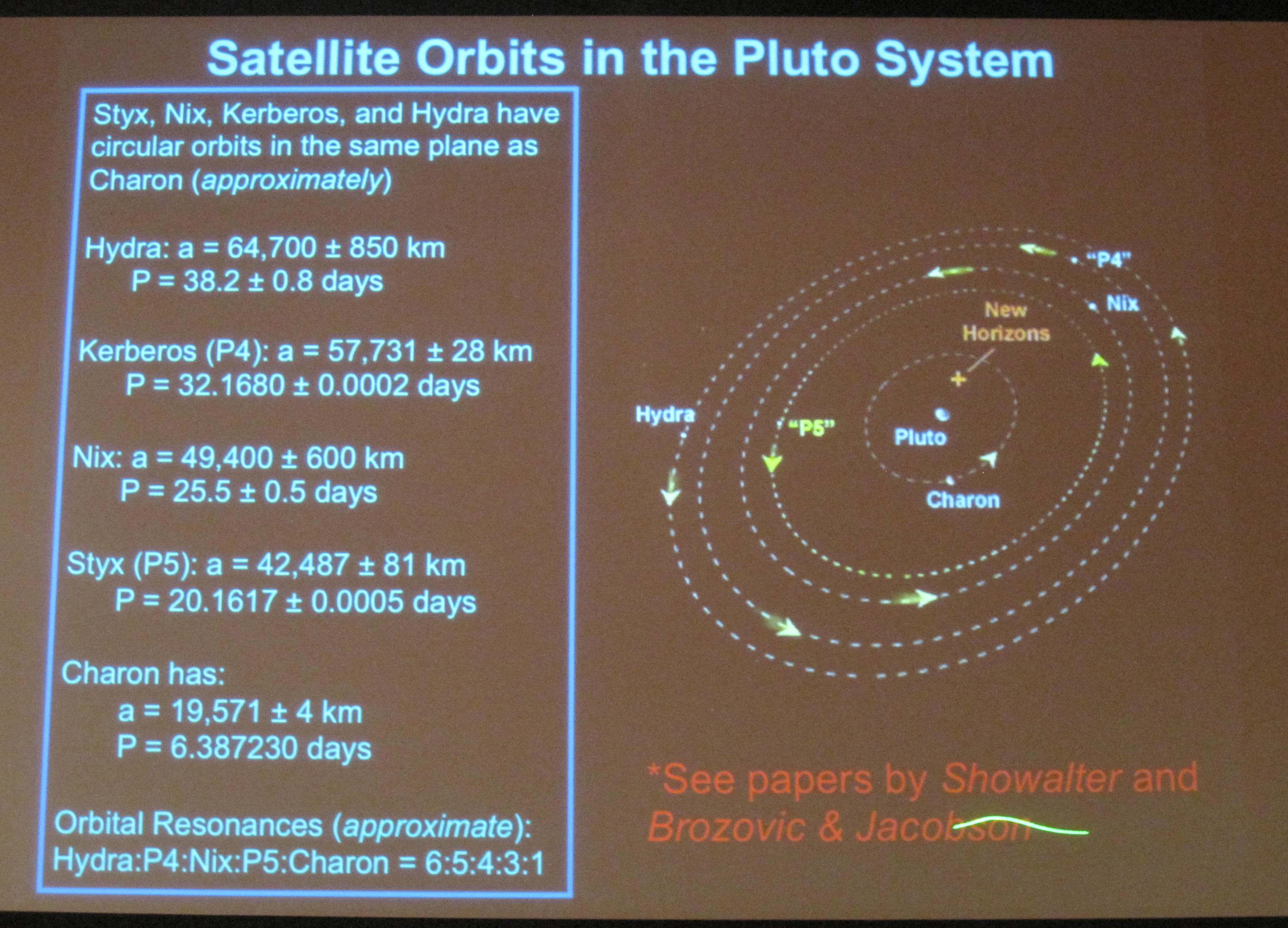
The Pluto system at a glance. Key top-level parameters of the satellites a=semimajor axis (from the Pluto-Charon barycenter/center of mass) in kilometers, P=orbital period in days. The moons appear to be in orbital resonances Hydra:Kerberos:Nix:Styx:Charon = 6:5:4:3:1.

What about their albedo? Albedo is a measurement of a body’s reflectance, a reflection coefficient, where an albedo equal to 1 is “white” and an albedo equal to 0 is essentially “black” (e.g., dirty snowballs like comet nuclei have albedos ~0.04). It should be noted that albedo values can be functions of color (wavelength of light). We know that Pluto has an albedo ~0.5 and Charon has albedo ~0.35. Regolith exchange and dynamics agreements favor albedo ~0.35 for these small satellites, and assuming that density=1 (icy body).

What are implications of these small satellite discoveries? These questions were posed: (1) Pluto system is highly compact and rich, so are there more satellites not yet discovered? (2) Was there a giant impact origin of Pluto System? (3) Could rings also form? (4) Could other large KBOs have multiple satellites? (We know Haumea has 2 companions. Could there be others?).

What role will New Horizons bring? New Horizons will play a key role for small satellites, measuring their size and their shapes. Note: Additional occultation observations from Earth could reveal additional satellites and also provide measurements of their sizes, but not shapes.

New Horizons best spatial resolution of the small satellites is: 0.46 km/pix (Nix), 1.14 km/pix (Hydra), 3.2 km/pix (Kerberos), and 3.2 km/pix (Styx). Best estimates right now for the sizes of these bodies, assuming albedo 0.35, are Hydra 50 km, Nix 40 km, Kerberos 10 km, Styx 4 km. That translates to roughly ~44, ~37, ~3, and ~1 pixels across Hydra, Nix, Kerberos, and Styx, respectively.

At the time of Kerberos & Styx’ discovery, the New Horizons Mission Ops team had already designed the Pluto science sequence of observations to run aboard the spacecraft.  In the spirit of exploration,  the team had wisely reserved a few TBD (to be determined) observations that they now have placed observations of Kerberos and Styx that fit within the constraints. Firm flexibility at its finest.

Scott Kenyon (Harvard SAO, by phone) “Formation of Pluto’s Low Mass Satellites.” He and his team looked at both the giant impact (Canup) and capture (Roskol) formation paths for Pluto and Charon. They model a debris disk where viscous diffusion expands the disk, collisions circularize the orbits, particles experience migration, and satellites eventually grow. They found that lower mask disks take longer to reach equilibrium, do produce more satellites, and also produce the smaller satellites. Calculations with large seed planetesimals produce less satellites. Calculations also do predict 1-km size objects in large orbits (orbits beyond Hydra) in a diffuse debris disk.

For more details about their paper on the formation of Pluto’s low mass satellites is found here http://arxiv.org/abs/1303.0280.

What role will New Horizons bring? New Horizons can test these predictions if they discover more satellites when they look at the Pluto system on approach and departure.

Peter Thomas (Cornell University) and Keith Noll (NASA GSFC) provided a talk about “Pluto’s Small Satellites: What to Expect, What They Might Tell Us.”

Small satellites of planets: variety and dynamics role. We have a small selection of satellites of 20-100 km range (e.g. Metis, Amalthea, Thebe, Atlas, Prometheus, Pandora, Epimetheus, Janus, Hyperion, Phoebe and asteroids Mathilde, Eros, Ida). Best “comparatives” come from the Saturn family from amazing Cassini images, but these divided into two groups whether they are located within the ring arcs or not. Small satellites are irregular in shape, have high porosity (40-70% void space), weak (tidally fractured), crater morphology varies, regolith depths & distribution over surface, icy & rocky, and some have albedo markings.

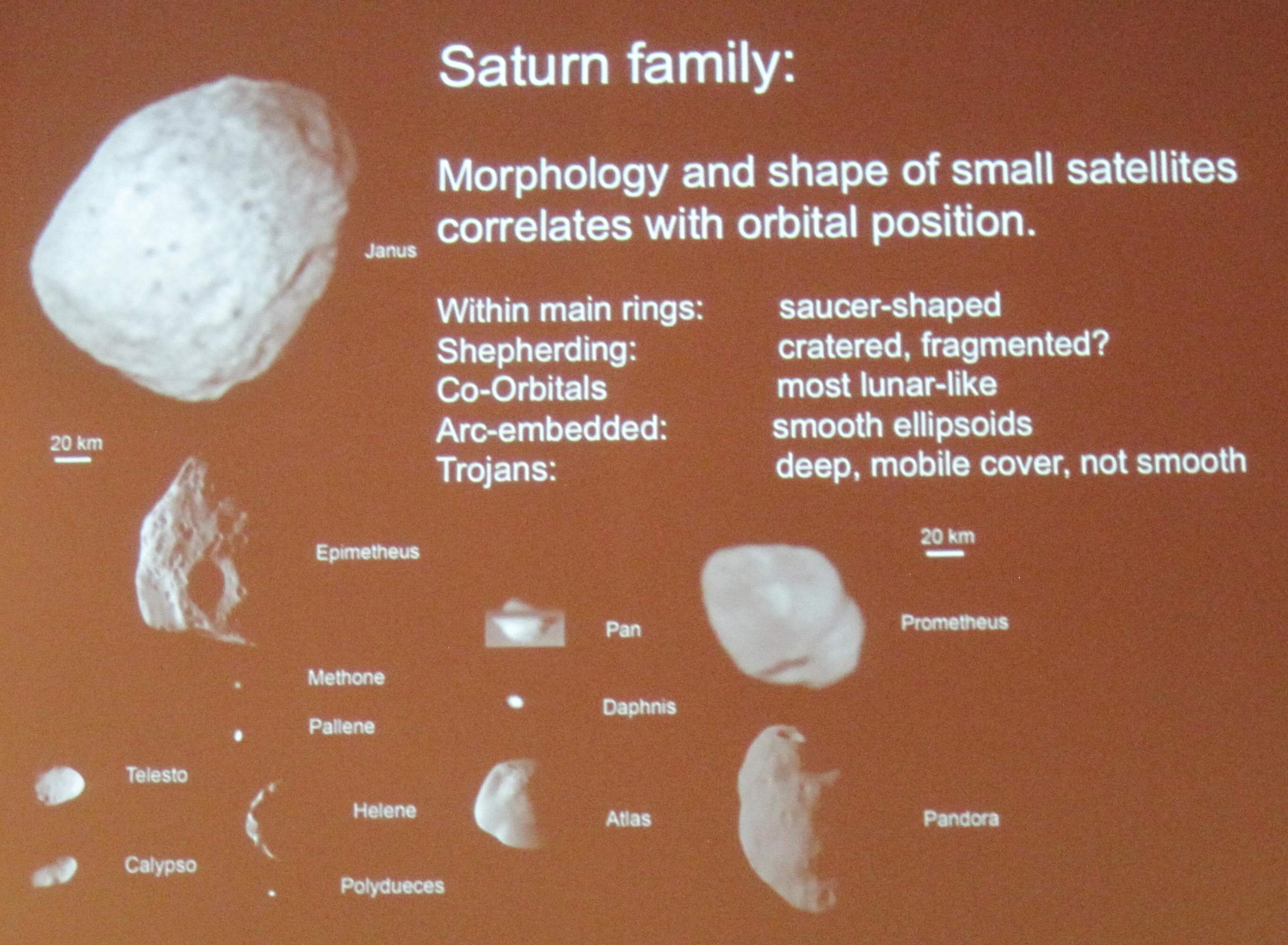
Saturn’s moons may be useful “comparatives” for describing Pluto’s small satellites.

Predictions for New Horizons. Peter Thomas is excited to see New Horizons’ images of the small satellites. He predicts they will not look like egg-shaped. Thomas’ Best Guess: A Deimos/Hyperion hybrid morphology.

KBOs and their satellites: variety and collision role. There are three multiple systems known in the Kuiper Belt: Pluto (6 components), Haumea (3 components) and 47171 1999 Tc36 (3 components). There are also 74 binary systems to date. The Pluto system is collisional. Unfortunately most of the KBO binaries have too low angular momentum to imply a collisional origin, but there is a subset of TNO binaries that could be a comparative set. Multiple collision systems in the Kuiper Belt could serve as possible analogs of the Pluto system.

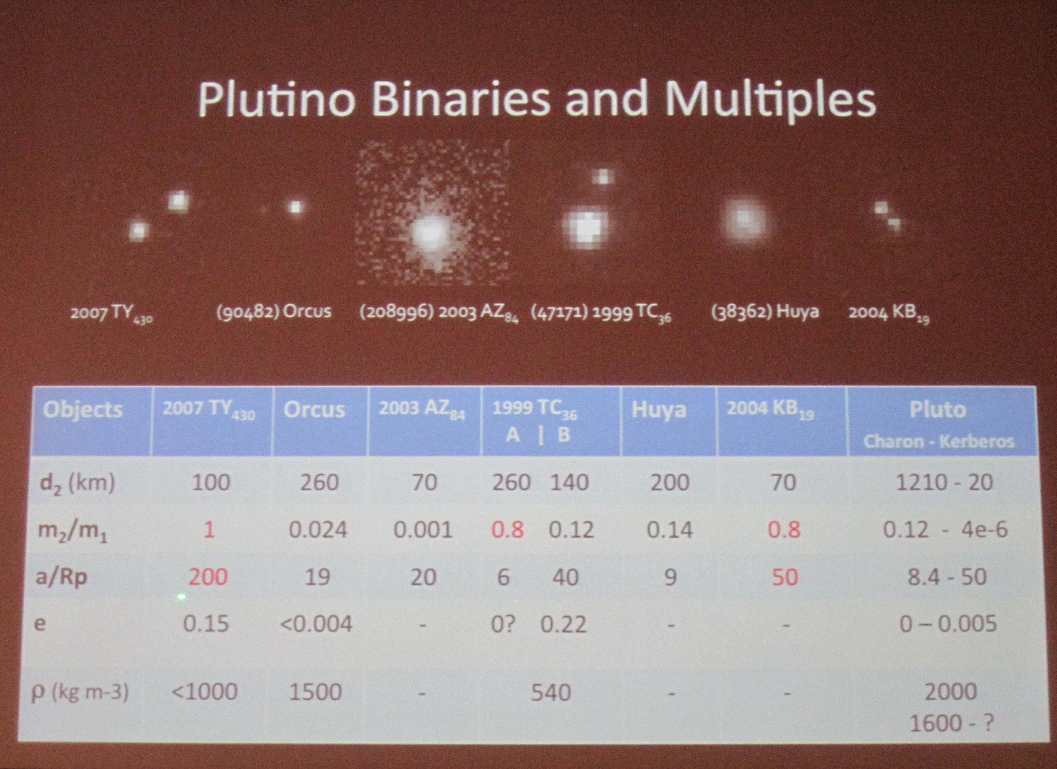
Plutino binaries (above) are also “comparatives” images for describing Pluto’s small satellites. Other comparative bodies, which may have collisional origin could be Quaoar, 1998 SM165, Salacia, and Eris.

Predictions for New Horizons. New Horizons will tell us a lot about KBOs and test open theories about their formation and collisional history.

Mark Showalter (SETI) on “Orbits and Physical Properties of Pluto’s Small Moons Kerberos (P4) and Styx (P5)” began with “Well, they are not your typical orbits.” The orbits of all the small satellites do wobble with a periodicity defined by Charon. Essentially the system acts like a “time-variable center gravity field.” There are nine orbital elements to fit (semi major axis, a; mean longitude at epoch, theta; eccentricity, e; longitude of pericenter at epoch, w; inclination I; longitude of ascending node at epoch, Omega; mean motion, n; pericenter precession rate dw/dt; nodal regression rate dOmega/dt.). He provided updated parameters for the moons based on this work.

Mark Showalter (SETI) next talked about his preliminary work on “Chaotic Rotation of Nix & Hydra.” He started the presentation with a light curves for Hydra & Nix made the 2010-2012 HST data sets. They do not follow the expected “double sinusoidal.” When plotting phase angle vs. time, Hydra and Nix do get brighter with lower phase angle and he used this information to normalize their light curves. He found that Nix & Hydra’s brightnesses do not correlate with their projected longitude on the sky. They are probably not in synchronous rotation. Also, he is not finding any single rotation period compatible with the data series he has.

His premise is that Nix and Hydra are not following your typical rotation, and are very heavily influenced by the Charon-wobble. Best Guess: Hydra and Nix are in a state of “tumbling.” Bodies that not synchronous have no way to get to synchronous lock.

Until now, Hyperion (one of Saturn’s moons) had been the only chaotic rotator. Not any more! It’s got company!

Marina Brozovic (JPL) spoke about “The Orbits and Masses of Pluto’s Satellites.” She used Pluto & Charon data from photographic plates (1980s), ground-based VLT AO data (1990-2006) and HST data (1990-2012); Nix and Hydra data from HST and VLT AO (2002-2012); and Kerberos and Styx data from HST (2010-2012) to derive orbital parameters for these bodies. They have created plu041 and plu042 ephemeris solutions (i.e. where all the satellites are in the system with time), the latter where they provide orbit predictions for the four smaller satellites. And, they have found interesting puzzles as they are working to find solutions for the new satellite masses. She presented orbital uncertainties at the time of the New Horizons encounter (July 14, 2015).

Andrew Youdin (JILA, CU Boulder) “Using (the stability of)  Kerberos to Weigh Nix & Hydra.” He looked at what was done on the HR8799 (Skemer et al 2012) exoplanet system, where orbital stability technique was used, and applied it to the Pluto System. Kerberos/P4 does appear more unstable, but Styx/P5 may be more stable. To derive the necessary masses for orbit stability, when compared with measured brightnesses, means comet-like albedos are ruled out for small Pluto satellites. Instead, they would have high albedo, clean-icy surfaces. No dirty snowballs here.

Andrew Youdin’s paper on using the P4 data to help constrain the masses of Nix and Hydra can be found here: http://arxiv.org/abs/1205.5273.

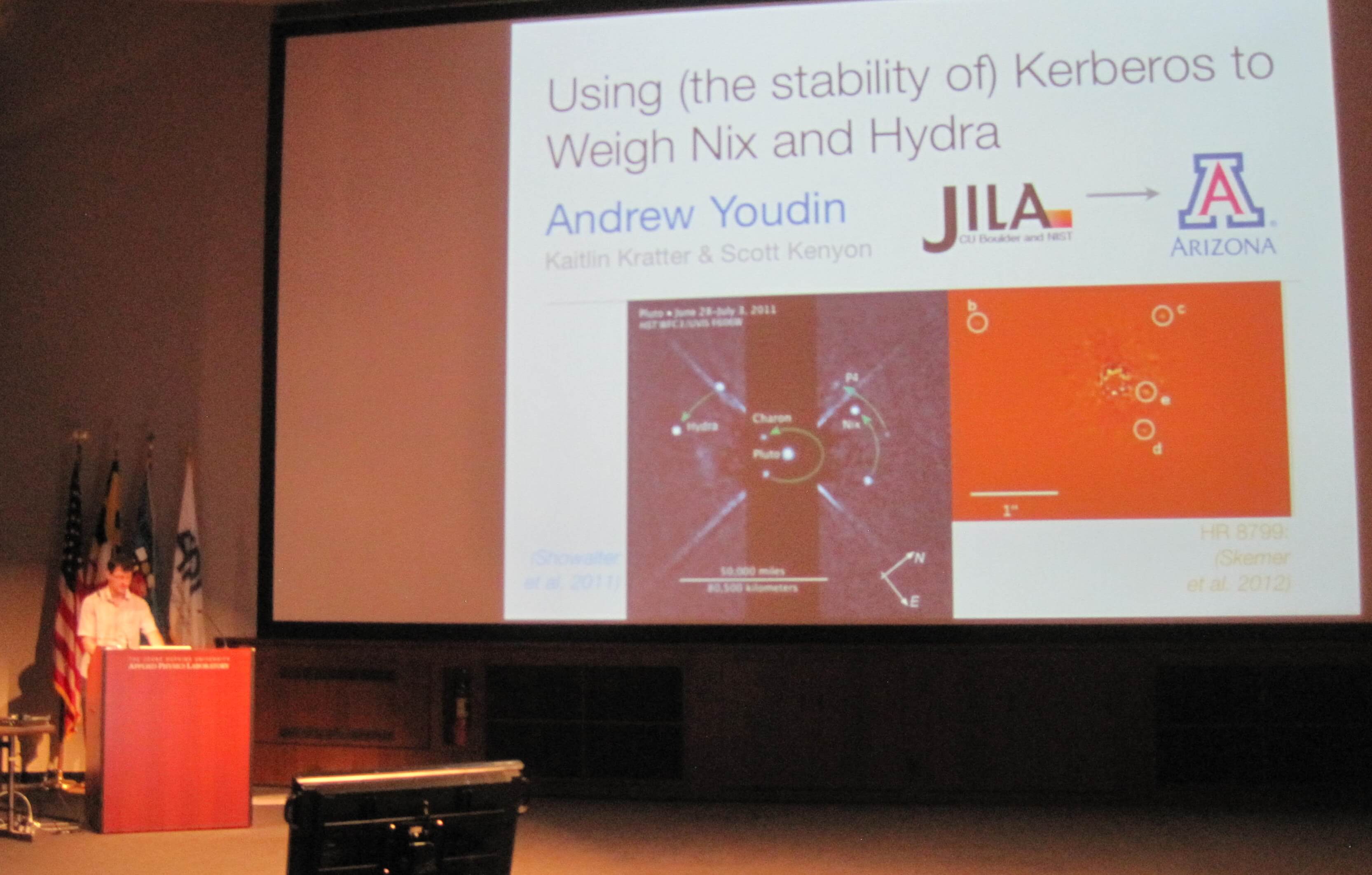
Andrew Youdin at the beginning of his talk called out a visual comparison between the Pluto System (left) and the exoplanet system HR8799 (right) 129 light years away characterized by a debris disk and four massive planets confirmed by direct imaging. It served for his inspiration to apply fitting. techniques to the Pluto System small moons. “Pluto’s not a planet. It’s better. In miniature, it’s the richest circumbinary multiplanet system.”

Alan Stern (SwRI) on “Constraints on Satellites of Pluto Interior to Charon’s Orbit and Prospects for Detection by New Horizons.” Alan Stern asks, “Could there be moons inside Charon’s Orbit?” Charon is a big vacuum cleaner, and clears out a big swatch called the CIS, the Charon Instability Strip, clear down to 0.45-0.47 Pluto-Charon separation. Atmospheric drag by Pluto’s atmosphere could also add in the clearing-out the region. Charon’s eccentricity also constrains the problem. And when you combine the recent HST data detection limits, you only have a region from 0.2 to 0.45-0.47 Pluto-Charon separation (the outer edge of the CIS) where youcould possibly have moons.

What role will New Horizons bring? New Horizons will do a deep satellite search with the LORRI instrument at seven days prior to Pluto closest approach. This search will reach 6x fainter than current limits set by HST for Pluto companions, to detect objects down to ~1.2 km. If New Horizons does find satellites within Charon’s orbit this will provide new insights into satellite system origins.

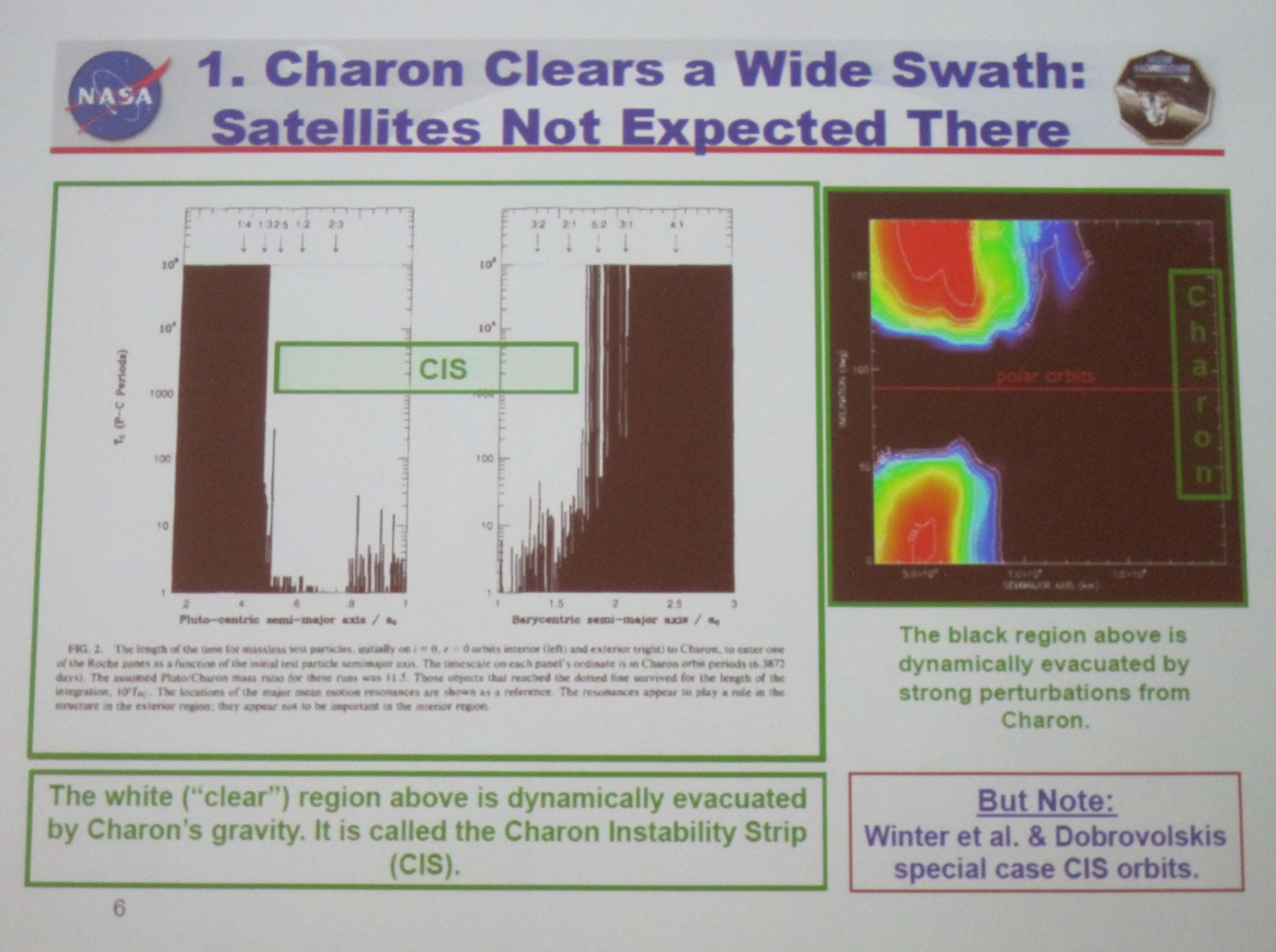
Charon has been a major player in the determining where debris in the Pluto system could remain stable. The Charon Instability Strip is a region between Pluto and Charon that is kept relatively free because of Charon’s gravity.

How can you form Pluto and Charon? Let me just count the ways.

Reposted from https://blogs.nasa.gov/mission-ames/2013/07/24/how-can-you-form-pluto-and-charon-let-me-just-count-the-ways/.

On the afternoon July 23, 2013 at the Pluto Science Conference continued, we switched gears from atmospheres to small satellites. This blog entry is about the formation theories for Pluto and Charon.

Hal Levison (SwRI) started the afternoon with a talk entitled “Unraveling the Early Dynamical Evolution of the Outer Solar system.” The “Nice Model” (Gomes, Levison, Morbidelli, Tsiganis) was devised to introduce possible models that could produce the Outer Solar System as we know it and preserve the Inner Solar System as we know it. The authors have been updating it with planets in resonances (Morbidelli et al 2007), put Pluto-objects in the disk (Levinson et al 2011), restricted the models to “save the Earth” by making sure Jupiter does not encounter an ice giant planet (Brasser et al 2009), and added a third ice giant (Nesvorny & Morbidelli 2011).

To learn more information about the Nice Model, check out a good entry at http://en.wikipedia.org/wiki/Nice_model.

The Nice model has told us a lot of good things. It predicts the right number and range or orbits for Jupiter and Saturn, predicts the right number and orbits for Trojans (things in 1:1 resonance with primary body) and reproduces the Late Heavy bombardment of Moon. However, it comes short of explaining the Kuiper Belt.

So, what does this all mean for the Kuiper Belt? The Kuiper Belt is a rich structure. Observationally the sum of all the mass in the Kuiper Belt is <= 0.1 Mass_Earth.  In order to get objects the size of Pluto to grow in the timescales of our Solar System, you need a lot more mass. So we need find this missing mass.

Above is a Comparison of updated 2008 Nice Model (green ) vs. Kuiper Belt Data (blue dots). It qualitatively shows similarities however it cannot reproduce the “kernel” (described in Brett Gladman’s talk from July 22nd) nor objects with high inclination (large i) nor objects in the “Cold Classical Population.”

Cold Classical Kuiper Belt Objects have orbits much like the planets; nearly circular, with an orbital eccentricity of less than 0.1, and with relatively low inclinations up to about 10° (they lie close to the plane of the Solar System rather than at an angle). They have characteristics similar to an undisturbed protoplanetary disk. Often the term ‘primordial’ is used when describing Cold Classicals. They tend to be in binaries and have “red” colors.

He then ended his talk by sharing an recent update with his work on Outer Solar System modeling, hoping to explain high inclination Kuiper Belt Object formation, by looking at the formation of Jupiter and Saturn with and without a gas disk present. Jupiter and Saturn, when they are forming, are scattering objects outward. Then if there is a gas disk present, these objects get into what is known as Kozai resonances, where bodies exchange eccentricity for inclination. As the gas disperses, a population at high inclinations in the Kuiper Belt region (30-50 AU) are caught. In the models, if you vary the outside extent of the disk, you spread out the populations. However, this is not in agreement with our solar system (we don’t see those types of objects). Their conclusion is that you needed to have the gas disk truncated and this modification of the Nice Model can explain high inclination KBOs.

Hal Levinson stated strongly “We definitely need New Horizons to visit a cold classical object!”

Anders Johansen (Lund University, Sweden) in “Accretion of Kuiper Belt Objects” stepped us through the two models of major planet formation: Planetesimal (coagulation) vs. Pebble (steaming instability).

He asked, could Pluto be formed by planetesimal accretion? This will require a cold disk of km-size planetesimals (Kenyon & Bromley 2012) where a key prediction of the planetesimal accretion model gives a differential size distribution that is in agreement with observations (i.e. lots of smaller objects). But, there is a problem this this approach since to make kilometer size objects beyond 20 AU as it would taken 100 Myr which is much longer than the life-time of the gas disk (Lambrechts & Johnansen, in prep). Thus, to make a Pluto-size (few 1000s km size) object would taker longer than the age of the Solar System. (Pluto orbit is 29 AU at closest to Sun to 49 AU, furthest from Sun). However adding streaming instability can speed up the planetesimal growth timeframe.

Could Pluto have been formed by pebble accretion? Pebbles are accreted very efficiently by planetesimals (Lambrechts & Johnansen,  2012; Ormel & Jlahr 2010). This shapes the distribution (makes it steeper) and brings it more into agreement with asteroid and KBO populations.

What new data will New Horizons shed? If data from New Horizons reveals the presence of Aluminum 26, this will imply a formation age for Pluto. Formation time data can be fed back into planet-forming models, be they planetesimal or pebble accretion, and those models can be used to help explain other systems, such as observed proto-planetary disks or exoplanet systems around other stars.

Robin Canup (SwRI) talked about the “Origin of Pluto’s Satellites.” Massive Charon and four very tiny outer moons make up Pluto’s satellites. All of these satellites are co-planar (they are moving in the same plane) and prograde with respect to Pluto’s rotation (they revolve about Pluto in the same direction as Pluto’s rotation). However, Pluto’s rotation is retrograde (in the motion opposite) to its orbit.

It is thought that Charon was formed by a giant impact that could have preserved a lot of angular momentum in the system. Her models (Canup 2011) predict a grazing impact was needed to match the system angular momentum and produce a Charon-mass object. Achieving a Charon-mass object requires an extreme case, as most of them like to create a companion that is 6-8% of mass of the primary object.

She also modeled cases where there is an undifferentiated impactor, and those systems can form “intact-moons.” In many scenarios, Charon-mass objects are created. And “the Charon that was created” forms entirely from impactor material. She postulates that this is the more probable explanation for Charon’s formation.

What about the origin of the tiny moons? The models do create a disk, which has enough mass to form tiny moons. The challenge is that the disk that is made too compact compared to the current existence of Nix & Hydra. Could these moons have been transported out? But no model has been able to drive them out via “resonant transport.”

The alternative theory for the formation of the smaller moons is by capture, but it’s rather very low probability. Plus that could imply far more irregular satellites and Pluto’s smaller moons are more regular. So this opens up the path for other theories. Collisional spreading? Collisional dampening? Preferential re-accretion?

This is an active area of study.

How New Horizons can help. By providing better constraints on masses and densities of Pluto & Charon, compositions of the tiny moons, any information about the differentiation shape of Pluto & Charon, and presence of distance satellites can better constrain these origin model.

More predictions about Pluto’s changing atmosphere. And Charon may have a few surprises of its own.

Reposted from https://blogs.nasa.gov/mission-ames/2013/07/24/more-predictions-about-plutos-changing-atmosphere-and-charon-may-have-a-few-surprises-of-her-own/.

Blog series continues. These are summaries of talks presented on July 23, 2013 at the Pluto Science Conference. The New Horizons mission will fly by the Pluto System on July 14, 2015, a place that has never been explored before by any other spacecraft. Many questions about the Pluto System remain unanswered. For more information about NASA’s intrepid explorer to the Solar Systems’ Third Zone go to http://pluto.jhuapl.edu/ and http://www.nasa.gov/mission_pages/newhorizons/main/index.html.

Richard French (Wellesley College) presented a talk on “A Comparison of Models of Tides in Pluto’s Atmosphere and Stellar Occultation Observations.”

We have come to understand that Pluto’s atmosphere is cold & tenuous, has a long radiative time constant, shows weak diurnal variations, indicates seasonal transport of volatiles with long term variations of atmospheric mass, and seems to be convectively stable. Current Pluto general circulation models (GCMs) predict smooth T(P) profiles reveal mean circulation and thermal structure. But there are problems. GCMs predictions (with these smooth T(P) profiles) are inconsistent with stellar occultation data, which imply much more complex T(P) profile. The other challenge to this mystery is that stellar occultations are spatially constrained (i.e., map across a particular lat/long swath of Pluto surface at the time of event).

Are there waves in Pluto’s atmosphere? This is one proposition to explain the structures (spikes) seen in the Pluto occultation data. Tidal models they have built make predictions for large scale and small-scale structures. Also they can predict temperature profiles with altitude. Next steps are to apply this model to other occultation geometries. Richard French showed a comparison of a tidal model (Toigo et al 2010) against occultation data from an event on Aug 21, 2002 and they showed qualitative agreement.

Richard French’s predictions for New Horizons fly-by: When New Horizons provides a true frost pattern, they can input this into their models and generate large-scale and small-scale structures for comparison with actual New Horizons atmosphere measurements. Their tidal models do generate regionally variable, latitude dependent thermal changes. If this is what New Horizons observers, their model can help constrain parameters.

Bruno Sicardy (Observatoire de Paris, France) next took us on a rich tour of “Pluto’s Atmospheric Pressure From Stellar Occultations: 2002-2012.”

There was a dual Pluto & Charon occultation event on 4 June 2011. Pluto and Charon each pass in front of the star (at different times). Look at curve shapes. Charon’s curve sharply drops, indicative of no atmosphere, unlike Pluto’s curve, which has not-as-steep ingress/egress that indicates the presence of an atmosphere.

Using the light curve data, Sicardy and his team use a temperature vs. altitude model to fit the light curve depth, width and ingress/egress slope. Then with the temperature, they can derive a pressure. He presented results from the most recent Pluto occultation that was observed May 4, 2013. Good data and good fit. Next were shown the derived pressure (at 1215km) for occultation events observed from 1988 to 2013.

]

Occultation results show the Pluto atmosphere is increasing over the past few years. There is some notable evolution and implies a regular expansion. But a question from the audience stressed caution as we could be seeing just the northern pole facing the Sun with that contributing to the expansion but it could be a localized phenomena.

Bruno Sicardy’s predictions for New Horizons fly-by: Atmosphere will be present for the fly-by.

Michael Person (MIT) next described “Trends in Pluto’s Atmosphere From Stellar Occultations.” He started his talk with the advantages of occultation measurements:  you get spatial resolution (~1 km at Pluto) with direct measurements of atmospheres (temperature, pressure, number profiles). MIT has collected data sets from 1988 through 2013. Their group tends to separate the upper vs. lower atmosphere when they fit their data. He next showed a light curve comparison over. Are we seeing a gradually decrease lower atmosphere slope? Is there a gradual lowering of the separation boundary?

“Haze or No Haze? That is the question.” Best evidence of haze is from the occultation event of 2002, where there is a distinct change in brightness as a function of wavelength (Elliot et al 2003).  Attempt to look for haze in the 2011 occultation event with SOFIA in three bands was not successful. The main question is why does the haze come and go, and what is causing it?

What Mike Person is looking forward to: New Horizons will finally provide the size of Pluto! Knowing where the Pluto surface really is, or equivalently, the size of Pluto, is a key data point, as all these interpretations of occultation light curves and interpretations to atmosphere assumes a Pluto size.

Alex Dias de Oliveira (Observatoire de Paris, France).“Pluto’s Atmosphere from Jul 18, 2012 stellar occultation.” This is his PhD work and he provided an updated status of the steps taken from prediction of the event, the observation data collected, various calibration items, and first attempts to invert the light curve to get a temperature profile. He observed this Pluto occultation event with the ESO VLT (8m telescope in Chile) with the NACO instrument in the H band (1.65 microns). Comparison with the June 12, 2006 AAT event showed that spikes seen in the light curves were repeated in the July 18, 2012 event he observed wit the VLT in Chile.

Cathy Olkin (SwRI) presented results from “The May 4th, 2013 Stellar Occultation by Pluto and Implications for Pluto Atmosphere in 2015.” This was an event where Pluto passed in front of a R=14.4 mag star with a slow shadow velocity of 10.6 km/s. The event was observed from the southern hemisphere, from Cerro Tololo in Chile.

Erika Barth (SwRI). “Is Methane Supersaturation Consistent with the Presence of Haze Particles in Pluto’s Atmosphere?” She asked the question: If you put haze particles into Pluto’s atmosphere how do they interact with the methane in Pluto’s atmosphere?” She developed a model to ingest haze particles into a supersaturated environment and this predicts the growth of clouds and condensation of methane. Then when methane condenses out, that reduces the amount of observable methane. Her model requires the existence of a troposphere (which we learned earlier in Emmanuel Lellouch’s talk today that there is no evidence for this, but its existence could explain some phenomena, some observed to date, other predicted) and also predicts a thick troposphere as well. She created a Pluto version of CARMA, the Community Aerosol and Radiation Model for Atmospheres.

Jason Cook (SwRI) next spoke about his “Analysis of High Resolution Spectra of Pluto: A Search for Cold Gaseous Methane Layer, and Spatial Variation in Methane Column Abundance.” Occultations have told us that Pluto’s upper atmosphere (above 1195 km) is pretty warm (100 K). But 2.15 micron N2 ice measurements of Pluto’s surface tells us the surface is ~40 K. So this implies there needs to be a cold-layer in the atmosphere. To investigate a search for this “cold layer of air” they took NIR (near infrared) spectra with NIRSPEC on Keck with R=35,000 in 2011. They need to move to a two-temperature model to help constrain the observed data (i.e. measured methane line depths from the high-res NIR spectra), but the hot/cold ratio of the two temperatures is an unresolved topic (pun intended).

They also took spectra of Pluto over several nights to probe the different longitudes of Pluto (Pluto has a rotational period of 6.4 days) and they got a fairly consistent number except near 180 deg longitude where gaseous CH4 was not easily detected. They would like more data to probe this temporal measurement.

Selection of high-resolution NIR spectra of Pluto obtained over several days. This series probes a range of Pluto rotations and show how methane lines (Q-branch) vary.

Eliot Young (SwRI) spoke about “Evidence for Recent Change in Pluto’s Haze Abundance.” Hazes have been observed on Titan (photolysis products from higher up in the atmosphere) and Triton (condensates from surface). The August 21, 2002 occultation showed evidence for haze (change in brightness with color, Elliot et al 2003), but 2007 (0.51 & 0.76 micron) and June & July 2011 occultation events in different bands (I & K bands) showed no change in color.

Occultations can only probe down to a certain depth, so they are limited. We don’t really how close you got to the Pluto surface. If you have a special case where you can have a central flash or sets of flash spikes, you can derive more information. By applying a new technique on the 2007 Mt John light curves, he proposed they can determine amount of haze by evaluating the attenuation in those parts of the light curve.

Central Flash Description:  A central-flash occultation is visible when the observer is located near the center of the shadow path of the object. It is here where the atmosphere near the edges of the occulting body (for Pluto occultations, this is Pluto) refracts extra star light (from the background star) directly opposite from the star, forming a “brightening” in the middle of the deep light curve.

Mark Gurwell (Harvard CfA) provided a talk entitled “Atmosphere CO on Pluto: Limits from Millimeter-Wave Spectroscopy.” Carbon monoxide (CO) is expected based upon the presence as an ice on its surface. The first direct detection of CO was done in the NIR with the VLT (Lellouch et al 2011). Then JCMT (Greaves et al 2011) revealed a CO(2-1) line in the submillimeter, but this line had not been there a few years back, leaving a mystery. There is still mystery in fitting the CO abundance based on the measured submillimeter width and strength of this line. He did show that Pluto had been in the fore-ground of a galactic emission during the JCMT observations. He supposes that they had contamination. They did their own observations using the SMA sub-millimeter telescope multiple times and did not detect the CO(2-1) line in the spectra (they have upper limits). So he is excited about using the ALMA array that has 30-50x SMA sensitivity to really address the CO, nitriles and isotopes.

And the final talk of the morning Atmosphere session just could not leave Charon out of it.

Alan Stern (SwRI) “Cometary Impact Produce Transient Atmospheres on Charon.” Most scientists have come to accept that Charon does not have an atmosphere (see earlier posting in Bruno Sicardy’s talk showing the dual occultation event for Pluto and Charon in Jun 2011.) But he postulates what about impacts? Coming from the Kuiper Belt, impactors (assuming cometary-level amounts of volatiles) could provide volatiles to the surface to Charon and therefore creating a “nanobar” atmosphere on Charon. Similar events could lead to atmospheres on Kuiper Belt objects. Their modeling (Trafton & Stern 2008) predicts presence of N2, CO, Ar, CH4, with CO dominating after impacts, and N2 being the dominate species (in terms of amount).

Predictions for New Horizons. Duty cycle would be short lived so it will be rare if New Horizons catches this event. However, with smaller impactor sizes, there could be a possibility that those events could have occurred within the “photoionization time” (before the molecule breaks down or escapes) or resulting implanted molecules by the time New Horizons gets there. Alan Stern coyly stated, “could be as much as a 25% chance” to see an nano-bar atmosphere on Charon.

A good question regarding surface volatiles that are revealed by impacts got the crowd excited. After all, when you describe an atmosphere you can categorize things as sources and sinks. Sources bring material to the system and here they could be not only the KBO impactor but also the materials that are revealed from the impacted-body after the impact.

On July 14, 2015 New Horizons will be doing a very sensitive experiment via the observations of the Charon occultation (Charon passing in front of our Sun as viewed from New Horizons).

Charon may indeed hold a few surprises of her own!

Pluto’s uppermost atmosphere. How big is it?

Reposted from https://blogs.nasa.gov/mission-ames/2013/07/24/plutos-uppermost-atmosphere-how-big-is-it/.

This is a blog series about talks presented that Pluto Science Conference, held July 22-26, 2013 in Laurel, MD.

Darrell Strobel (JHU) next took us through a study about  “Pluto’s Atmosphere: Escape and the Relationship to Density and Thermal Structure.”

But first, what hydrodynamic escape discussion could be complete without a few equations….

Yes, this is what an atmospheric modeler solves for. He/she solves numerous energy-balance, energy-transport, etc. equations to derive properties for making an atmosphere.

The Hydrodynamic escape rate is a key output from these numerical models for Pluto, with predictions in the range of 1.5-6.7 x 1027 particles/s. The basic problem with computing hydrodynamic escape is due to the presence of a gravity well that these molecules need to escape from. Essentially, you need an additional energy input (such as thermal) to drive the escape process.

Some other key terminology: “The exosphere is a thin, atmosphere-like volume surrounding a planetary body where molecules are gravitationally bound to that body, but where the density is too low for them to behave as a gas by colliding with each other.” (Wikipedia) It is the uppermost layer where the atmosphere thins out and merges with interplanetary space. Theexobase is the lower boundary of the exosphere, defined as the altitude at which the atmosphere becomes collisionless.  Atmospheres can lose atoms from stratosphere, especially low-mass ones, because they exceed the escape velocity (Ve= (2GM/ R)½). This is known as (Jeans escape or Thermal Escape). The Jeans parameter (lambda) is a measure of how efficient the loss mechanism is. Larger lambda values implies less loss (smaller escape rates).

Models by different groups predict Pluto’s exobase between 5 and 10 Pluto radii. Assuming Pluto radius of 1200 km, Pluto’s exobase is in the 6000-12,000 km range. New Horizons’ nominal trajectory will bring the spacecraft to within ~10,000 km of Pluto’s surface and ignoring the slight fact that there are uncertainties in deriving Pluto’s size in the 20-100 km range and ignoring whether you determine a planet size by including or excluding the atmosphere, there is a possibility New Horizons could be flying through Pluto’s exosphere. Such an extended atmosphere could be affected by Charon and could affect Pluto’s interaction with the solar wind at the New Horizon encounter, as measured by New Horizons instruments PEPSSI and SWAP. (For more talk summaries about solar wind, see later blog entry).

A plot of temperature in Kelvin (x axis) vs. altitude in km (y axis) is a typical output of this type of model. Below is a particular plot shows the effect of adiabatic cooling, which Darrel Strobel stressed, is a key component that cannot be ignored. Another key output from these models is the computation of number density (N2 molecules/cm2/s) as a function of altitude.

Temperature profile with altitude for models with (blue) and without (red) adiabatic cooling. The surface is at 40 K (which is from observation evidence) and upper atmosphere temperatures are in the 100s of Kelvin (supported by NIR spectral observations of methane). The two models predict wildly different temperatures at high altitudes depending on whether cooling is occurring.

Darrel Strobel’s predictions for New Horizons fly-by: Escape rate 3.5×1027 N2/s, exobase at 8 Rpluto ~9600 km, Jeans Parameter Lambda ~ 5.

Weather on Pluto. Fair, haze patches at first. Moderate calm with the occasional chop.

Reposted from https://blogs.nasa.gov/mission-ames/2013/07/24/weather-on-pluto-fair-haze-patches-at-first-moderate-calm-with-the-occasional-chop/.

The July 23, 2013 morning session of the Pluto Science Conference started with a collection of talks addressing what we know and what we don’t know about Pluto’s atmosphere.

Emmanuel Lellouch (Paris Observatory, France) spoke about “Pluto’s Atmosphere: Current Knowledge and Open Questions.”

What do we know about Pluto’s Atmosphere? We know that it is a nitrogen (N2) dominated atmosphere with methane (CH4) (tens of %) and probably carbon monoxide (CO). It’s about 10-microbar (pressure) class showing evidence for changes in pressure on year/decade timescales. There is also evidence for waves (dynamic changes), and the atmosphere does have a thermal structure, despite the details being hotly debated in the community (pun intended). People do agree that the surface is cold (40-50 K) and then the atmosphere is around 100K at micro-bar pressure levels. The details of the cold/warm layers in between are the stuff that thermal models are made of!

Pluto was discovered in 1930, but it was only in 1985 that the first observation detecting an atmosphere around Pluto was made. It was discovered through a measurement called a stellar occultation, when Pluto crossed between a star and an observer on Earth, on August 19, 1985 (Brosch, MNRAS, 1995). A higher signal-to-noise light curve was obtained on the June 9, 1988 (Elliot, et al 1989) occultation events whose light curves indicated existence of waves.

Occultation light curve for Pluto passing in front of a star on June 9, 1988 (signal vs. time) Features in this dataset indicate the upper atmosphere (above the ‘kink’) and lower atmosphere (below the ‘kink’). The ‘kink’ presence is theorized to be due to heating by methane (Hubbard et al 1990). Waves are indicated by the “spikes” in the light curve. When the scientists create this light curve from the occultation event, they then “invert” it to fit a temperature model and derive pressures for different scale heights.

The first molecular detection of anything in the Pluto’s atmosphere was methane (L. Young et al 1997) using the IRTF (3.5 m telescope) in May 1992. This was confirmed and re-measured in 2008 with higher resolutions and sensitivity (Lellouch et al 2009) using the VLT (8 meter telescope) with more recent observations in 2012. Emmanuel Lellouch showed that with those two latter datasets there was no evidence of change in the last four years. With this higher resolution data they can use it to provide a fit to the temperature using the line widths.

Carbon monoxide (CO) was detected in the submillimeter at 240 GHz with JCMT (Greaves et al 2011), but this detection and the inferred amount has lead to questions that the current models cannot produce this molecule with the temperature and amount inferred from the observations. This particular topic was addressed by Mark Gurwell’s talk later in the morning.

There is also evidence for diluted methane (CH4) and pure CH4 ice on Pluto’s surface. The atmosphere CH4 is much greater than what is expected from an ideal mixture, so this implies there must be a mechanism to enrich the CH4 component in Pluto’s atmosphere. Recent thermo-dynamic models and “GCMs” (general circulation models) predict a consistent mixture for CH4.

The combination of both the infrared spectral results and the visible (and in some case near-infrared) occultation light profiles helps resolve temperature profile (i.e., how temperature varies with altitude) inconsistences.

Speaking of temperature profiles, one of the hotly debated topics for Pluto atmosphere specialists is whether their models contain a tropopause. Per Emmanuel Lellouch’s overview talk, he stated, “There is no proof there is a troposphere. And deep troposphere are not predicted by the GCMs.” However, many Pluto atmosphere specialists often invoke a troposphere in their calculations to help predict other things that have been inferred to occur on Pluto.

Pluto’s atmosphere seems to be changing. There is observation of pressure evolution. Specifically, the pressure appears to have doubled from 1988 to 2002 (Sicardy et al 2003, Eliot et al 2003). Evidence that the pressure is continuing to increase is based on recent 2013 occultation data. This has led to the development of Volatile Transport Models. These are basically computations that track the dominant species, and for Pluto, it is nitrogen, through multiple temperature and pressure ranges, heat exchanges such as sublimation cooling in summer and condensation heating in winter. A schematic of a Volatile Transport Model from Leslie Young, New Horizons deputy Project Scientist, is shown below.

Schematic of a volatile transport model for Pluto. More details about the model are in a blog on Leslie Young’s volatile transport model talk later in the conference.

Other Oddities in Pluto’s Atmosphere. There appears to be evidence for photochemical haze from a 2002 occultation (Elliott et al 2003) but occultations in 2007 and 2011 did not show evidence of this. Hazes are large particles in the atmosphere (almost cloud-like) and the 2002 occultation had suggested hazes since there had been a distinct change in brightness as a function of wavelength. Why does the haze come and go, and what is causing it?

Pluto has also indicated “reddening” (color-change) that occurred between 2000 and 2002 (Marc Buie using color photometry with HST). That’s a mystery.

Waves (dynamic changes) in atmosphere are indicated by some of the occultation measurements. What could cause waves? There are multiple suggestions what could form these dynamic changes (even evoking the elusive gravity wave mechanism). Could it simply be Pluto’s atmosphere response due to the diurnal variation of sublimation of N2 particles?

What will Pluto’s Atmosphere be like when New Horizons comes to take a close look?

  • Will the atmosphere be there in 2015? Lellouch’s best guess: Yes.
  • Will there be a thermal structure (i.e. see a troposphere)? Lellouch’s best guess: Hopefully (helps modelers out).
  • Will there be other gases present (i.e. C2H2 HCN, etc.)? Lellouch’s best guess: Maybe.
  • Will there be clouds or hazes? Lellouch’s best guess: Maybe.
  • When will the atmosphere collapse (i.e. pressure drops by orders of magnitude)? Lellouch’s best guess: “Your guess is as good as mine.”