The Pluto science community is rich and diverse, just like its target of study: the ever-fascinating Pluto and its satellite moons.

Reposted from https://blogs.nasa.gov/mission-ames/2013/07/27/the-pluto-science-community-is-rich-and-diverse-just-like-its-target-of-study-the-ever-fascinating-pluto-and-its-satellite-moons/.

This blog entry concludes my series of talk summaries for the July 22-26, 2013 Pluto Science Conference, “The Pluto System on the Eve of Exploration by New Horizons: Perspectives and Predictions.” You can read more about the conference and browse through the abstracts at the conference website.

In his closing comments, Alan Stern (SwRI), the lead scientist (Principal Investigator) for NASA’s New Horizons fly-by mission to Pluto, told us about the last time a scientific discussion gathering specifically about Pluto occurred. It was twenty years ago, a 3-day meeting in July 1993, in Flagstaff, Arizona. The talks and presentations from that workshop led to ten contributed papers in a special issue in 1994 in Icarus (Vol 108, Issue 2) and, in 1997, the publication of a book entitled “Pluto and Charon” by The University of Arizona Press.

When the group gathered in 1993, the 1989 Voyager 2 fly-by of Neptune’s moon Triton’s was still “fresh data”, the prime Pluto-Charon “Mutual Events Period” of the 1985-1990 had just ended, and the Hubble Space Telescope (HST) would be soon coming back on-line with its fixed optics (the 1st HST servicing mission would occur in December 1993). It was a busy time for the Pluto science community.

Some attendees at the open workshop meeting on Pluto & Charon in July 1993, Flagstaff, Arizona.

This five-day July 2013 meeting has demonstrated that the quest to better understand Pluto and its environment is a very rich and diverse field of study. With each new data set about Pluto and its companions, surprises are uncovered and new questions are posed. When the New Horizons spacecraft reaches the Pluto system in July 2015, a true “first encounter experience,” its on-board suite of modern instruments will transform our current-best resolution ~800 km/pixel (from Hubble observations) to a resolution of 0.46 km/pix (hemisphere) with 0.09 km/pix (regional) resolution with the LORRI instrument. You can be certain there will be a lot more surprises in store. Combining this with new and unique data sets from New Horizons’ particle & dust instruments and the UV and IR spectrometers, our understanding of the Outer Solar System will find a new grounding.

With 103 oral talks + 30 posters + 13 “topical sessions” this was a jammed pack week of sharing old information, sharing new data from the past few years, sharing “hot off the press data” (it’s Pluto observing season right now and during the conference attendees were doing observations of Pluto & Charon with IRTF, Keck and other telescopes, remotely or with their colleagues at the telescopes), identifying what computations or experiments are needed before the 2015 encounter, and in some cases, providing predictions of what might be detected at Pluto and Charon. Several papers presented at this conference will be submitted to the Icarus journal.

Attendees at the “The Pluto System on the Eve of Exploration by New Horizons: Perspectives and Predictions,” held July 22-26, 2013, in Laurel, MD. The topical sessions covered Atmospheres, Charon, Dust & Rings, Interiors, Kuiper Belt Context, Laboratory Studies, Magnetosphere, New Horizons Mission, Origins, Satellites, Surface Composition, Surface Geology, and Surface-Atmosphere Interactions.

The stage is set for a summer 2017 Pluto Science Conference. New Horizon’s flyby of the Pluto System is on July 14, 2015, but it will take a bit over a year for all the data to come down losslessly (i.e. without compression). Deliveries to the NASA’s Planetary Data System are planned in 2016 and early 2017.

I hope you enjoyed this blog series reporting on these intriguing topics. You can follow the New Horizons mission status at any time by visiting the New Horizons Mission Website at http://pluto.jhuapl.edu/ and http://www.nasa.gov/mission_pages/newhorizons/main/index.html.

To Pluto and Beyond!!!!

Pluto Exotica. Atoms. Pick Up Ions. Bow Shocks. Suprathermal Tails. X-Rays. UV airglow.

Reposted from https://blogs.nasa.gov/mission-ames/2013/07/27/pluto-exotica-atoms-pick-up-ions-bow-shocks-suprathermal-tails-x-rays-uv-airglow/.

The morning of the last day of this week’s July 22-26, 2013, Pluto Science Conference opened up the discussion with outer atmosphere (far out) and magnetosphere (really far out) talks.

Fran Bagenal (University of Colorado) started the session with a talk on “The Solar Wind Interaction with Pluto’s Escaping Atmosphere.” Pluto’s interaction with the solar wind was first suggested in 1981 by Larry Trafton. There are two generally predicted regimes of what this interaction might look like: (1) Venus-like (small escape rate) and (2) Comet-Like (high escape rate). A key parameter distinguishing the two is what the atmospheric escape rate might be, that is, how many atmospheric molecules (assumed to be nitrogen) are escaping from Pluto, no longer being bound by gravity. Current estimates for the escape rate, based on a number of approaches, notably a recent one by Darrell Strobel (2012), have this number at 2-5×1027molecules/sec.  This is large enough to suggest Pluto will appear to be “comet-like” in its interaction with the solar wind. However, we need to wait until 2015 for the New Horizons fly-by with their in-situ particle instruments SWAP & PEPSSI to make the interaction measurements.

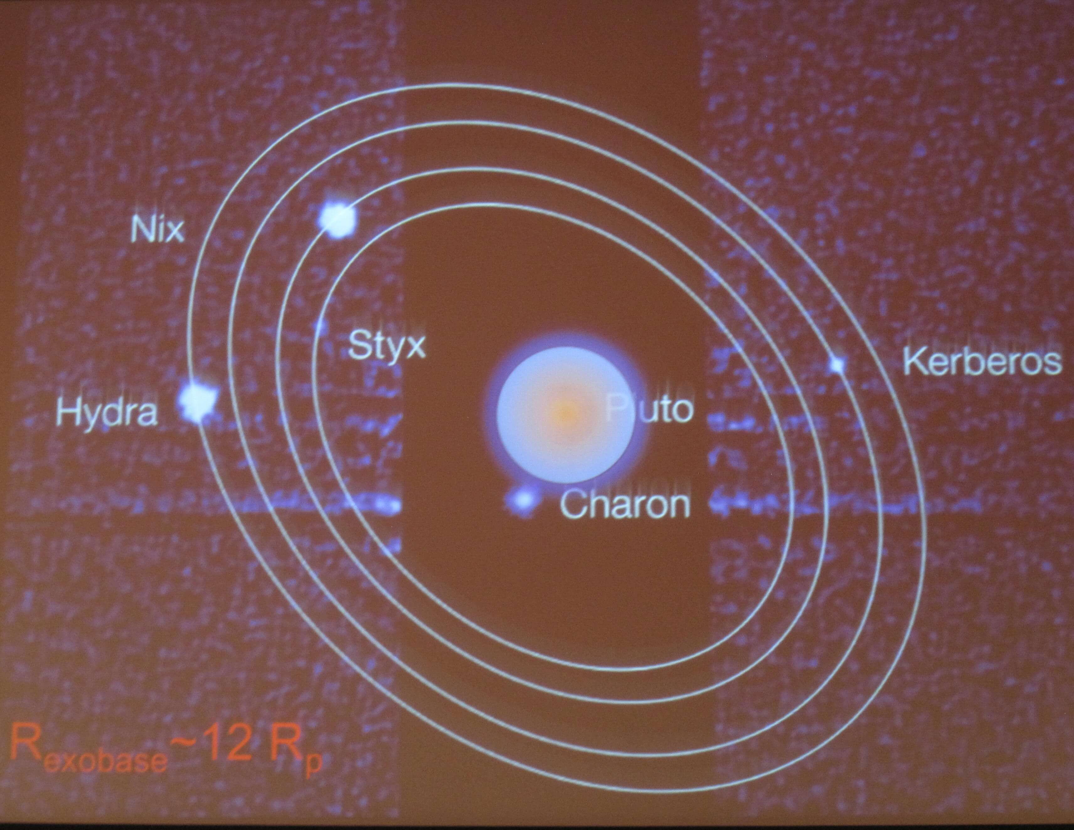
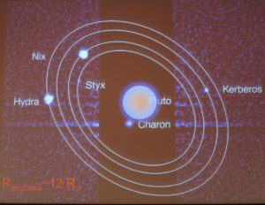
When describing the Pluto System in terms of solar wind interaction, Fran Bagenal showed this image, which superimposed one of Darrell Strobel’s atmospheres (characterized with an exobase at 12 Pluto radii). Pluto becomes a “large object” for interaction with the solar wind.

When solar wind particles (protons) interact with the Pluto atmosphere, their path through space is bent along the magnetic field lines, and to convert momentum, pickup ions (neutral hydrogen atoms from the heliosphere that undergo a collisional charge-exchange interaction with solar wind protons, get ionized, are “picked up” by the solar magnetic field) get tossed onto new trajectories. Those ions are charged and will begin to rotate and follow electrical field lines. Where do the ionized particles go? A weak magnetic field will create large gyro-radii of pick-up ions which can extend millions of kilometers upstream of Pluto.  This is best modeled with a kinetic interaction.

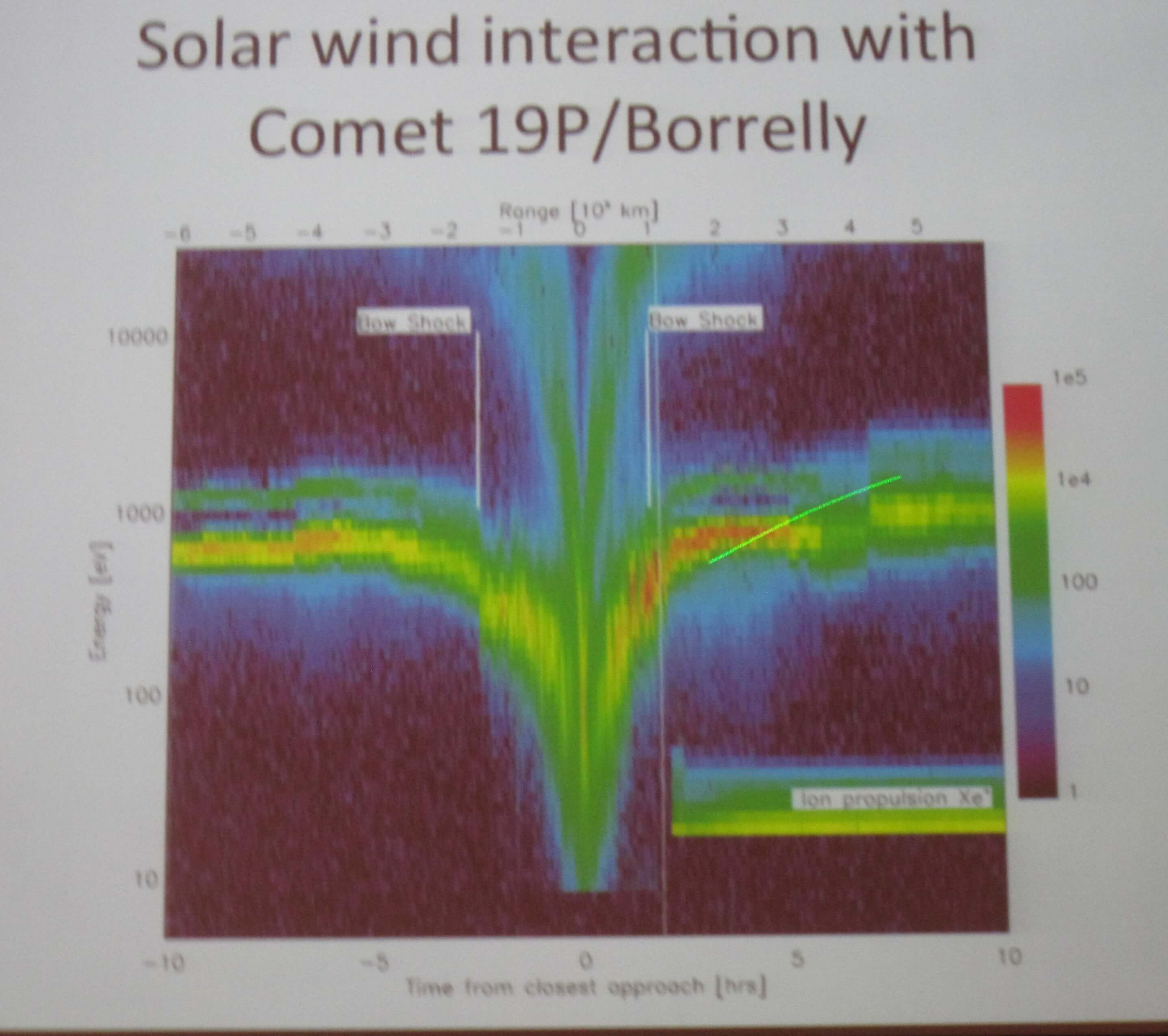
Peter Delamere (University of Alaska, Fairbanks) spoke in greater detail about “The Atmosphere-Plasma Interaction: Hybrid Simulations.” Plasma interaction is an atmospheric diagnostic tool. Neutral gases are not easily picked up, but ions and how they interact with the solar wind can be detected with in-situ instruments such Hew Horizons’ SWAP and PEPSSI. He discussed his model plasma interaction mode, which was validated using Comet 19P/Borrelly that had been visited by Deep Space 1 on Sept 22, 2001.

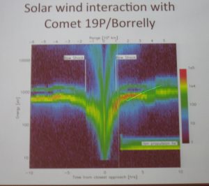
Example of Comet 19B/Borelly environment time vs. energy reveals the structure of the interaction between a comet and the solar wind. The X-axis is time from closes approach, with the Y-axis energy. The color code is the number of particles counted by the PEPE instrument aboard Deep Space 1. This is similar to what the data is expected to look at for Pluto when New Horizons reaches it in 2015, however, the solar wind at 33 AU may be more extended and more diffuse and therefore the signal strength (in terms of counts) will be much less.

If we can understand where the bow shock forms, this becomes a diagnostic of the atmosphere, and if indeed the exosphere extends out to 10 Pluto radii as suggested by recent work by Darrell Strobel (2012) and other models, then this is a sizable ‘obstacle.’ But is it inflated enough to form a bow shock? Peter Delamere thinks so. He stepped us through a variety of simulations. One of the simulations predicts a partial bow shock. If you increase Qo (the escape rate parameter, predicted to be in the 2-5×1027 N2 molecules) or increase magnetic field strength you can create a full bow shock. Future work includes adding the pickup part of the solar wind model as input.  If there is a very slow momentum transfer, perturbed flow could extend out to an AU.

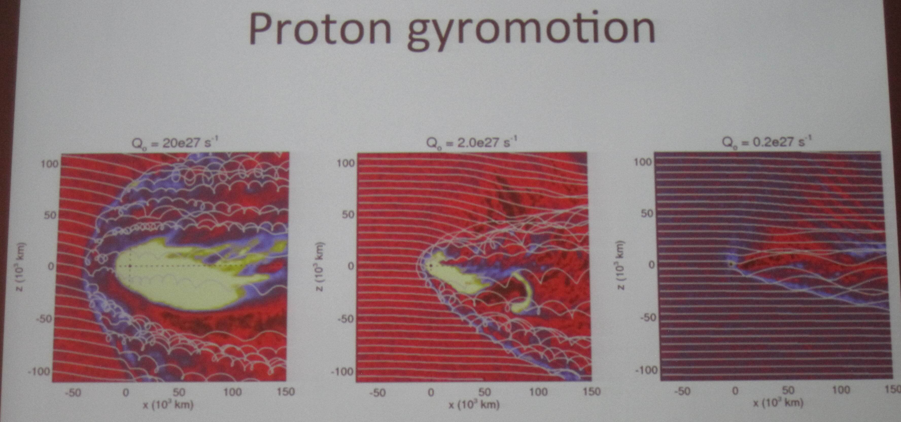
Simulations predict all sorts of shock structures (Mach cones, bow shocks), but these structures depend on the escape rate parameter.

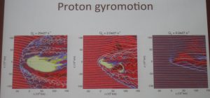
Example of a plasma interaction mode for three escape rates, decreasing from right to left. This is a slide in space of plane vs. distance from.  The white lines are sample solar wind proton trajectories. The color scale indicates ion density. The solar wind (and hence, the direction from the sun) is incident from the left. Pluto is at (0,0).

Predictions at Pluto. He anticipates significant asymmetry. The predicted bow show could be as far as 500 Pluto radii.

Heather Elliot (SwRI, San Antonio) in her talk “Analysis Techniques and Tools for the New Horizons Solar Wind around Pluto” described the New Horizons SWAP instrument and the different rate modes (sampling rate and scan types) it will be using during the 2015 encounter.

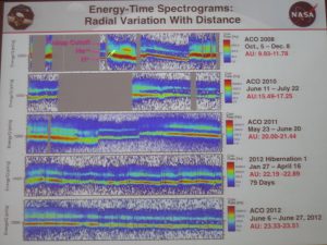
Measurement of the solar wind taken with the SWAP instrument aboard New Horizons during the last 6 years of cruise. This data set covers AU=10 (Saturn distance) out to AU=23 in 2012. The solar wind is mostly protons (H+). The second most abundant species are alphas (He++). The colors are the intensity of species. The vertical axes are energy per charge units and the horizontal axis is time.

Fitting the SWAP data to a solar wind model requires making adjustments for view angle and during the hibernation period, when they do not have attitude information, they have modeled the Sun-probe-Earth angle to estimate the attitude and this works well to fit their data.

John Cooper (NASA Goddard) spoke about the  “Heliospheric Irradiation in Domains of Pluto System and Kuiper Belt.”  He is interested in computing the “radiolytic” dosage onto bodies in the outer solar system (that is, the effect of how molecules break down or change molecular band structure due to the influence of radiation, such as by cosmic rays, particles, UV, etc.). For this he needs measurements of the particle flux at large AU.  New Horizons joins its cousins Voyager 1 & 2, Pioneer 10 & 11 and Ulysses in exploring the outer solar system.

spacecraft_outersolar

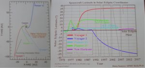
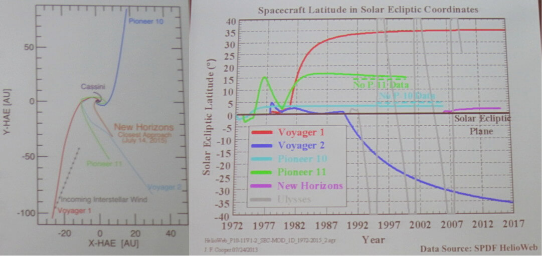
Location of the NH spacecraft (orange on the left, purple on the right) for two different views of the solar system. Also plotted are deep space missions Voyager and Pioneer, among many. The left view is s top down view of the solar system with the Sun at (0,0), the axes are in AU, where 1 AU (Astronomical Unit) is the distance between the Earth and Sun. The right is a view of time vs. latitude for the crafts. Comparative data sets to New Horizons, which travels along the solar ecliptic, are Pioneer 10 and early Voyager 2 data.

He showed computations of irradiation dosage when applying those particle rates measured by New Horizon’s PEPSSI instrument and instruments aboard Voyager 2 and Pioneer 10.

He maintains a database of all particle instrument flux measurements at the Virtual Energetic Particle Observatory http://vepo.gsfc.nasa.gov.

Thomas Cravens (JHU/APL) with ”The Plasma Environment of Pluto and X-Ray Emission: Predictions for New Horizons,” asked “What happens when you get to within 1000 km of Pluto?“  Pluto is anticipated to be “Comet-Like” in its interaction with the solar wind, however when you get closer to Pluto (around 1000 km), it may more closely resemble “Venus-like” interaction. He is trying to compute where the charge-exchange boundary could be, probably around r~5000km. This is boundary between the kinetic (r>5000km) and fluid (r<5000 km) regimes, essentially probing the ionosphere regime of Pluto.

Switching to slightly lower energies, Casey Lisse (JHU/APL) gave a talk on “Chandra Observations of Pluto’s Escaping Atmosphere in Support of New Horizons.” X ray interactions (charge exchange, scattering and auroral precipitation) require an extensive neutral atmosphere, which is what is expected at Pluto. Interaction of solar wind with comets has consistently shown X-ray emission. He expects to see X-ray emission from Pluto. If detected it would tell us about the size and mass of Pluto’s unbound atmosphere. The best time to look for x-rays at Pluto is about 100 days after a large CME (corona mass ejection) event, which is about the time it takes for CME to get to Pluto at 33 AU.

He and his colleagues applied for, and got, time on NASA’s Chandra X-ray telescope. On Chandra, Pluto & Charon will appear to fill one Chandra pixel using the Chandra HRC instrument.  He ended his talk suggesting that looking at background counts with the LORRI and RALPH CCDs might serve as a poorman’s x-ray detector. It is also possible that PEPSSI background counts could be used to infer presence of lower X-rays.

Kandi Jessup (SwRI) gave a talk addressing the “14N15N Detectability at Pluto.” We care about14N15N because it can be used to determine the 15N to 14N isotropic fractionation. This can help tell us about the evolution of Pluto’s atmosphere. Learning about Pluto’s atmospheric evolution history also provides vital suggestions for the evolution of equivalent TNOs (Trans-Neptunian Objects) and other objects in the Kuiper Belt, and hence, the outermost parts of our Solar System

The measurement will be the UV spectral observations during the solar occultation of Pluto by the Alice instrument during the New Horizons fly-by. N2 is the dominant absorber between 80-100nm. To identify the molecule 14N15N they use an atmosphere model from Krasnopolsky & Cruikshank (1999). That model does not have a troposphere. Next they need absorption cross-sections (a parameter that quantifies the ability of a molecule to absorb a photon of a particular wavelength) for 14N2 and 14N15N. 14N2 is the more dominant species and they are trying to find a very small percentage for 14N15N. Using these simulations they anticipate the Alice instrument will be sensitive enough to detect at least a 14N15N to 14N2 ratio of 0.3%. They will be look at the UV spectrum between 88 and 90 nm where the 15N lines spectrally shifted from 14N line. 14N15N to 14N2 ratio has been measured on Mars (0.58%), Titan (0.55%), and Earth (0.37%). What ratio will Pluto have? New Horizons data will hopefully tell us.

Randy Gladstone (SwRI, San Antonio) spoke about “Ly-alpha at Pluto.” Pluto ultraviolet (UV) airglow line emissions will be very weak, except at HI Lyman-alpha (Ly-a). Ly-a at Pluto could have both a solar (Sun) and an interplanetary (IPM/interplanetary medium) source. Ly-a should be scattered by Hydrogen atoms in Pluto’s atmosphere.  He uses the Krasnopolsky & Cruikshank (1999) Pluto atmosphere model that predicts the number of Hydrogen atoms at altitude. There are several observations near Pluto closest approach planned with the New Horizons Alice instrument to measure Lyman-alpha emissions.  This data will provide information about the vertical distribution of H and CH4 in Pluto’s atmosphere. Observation of the IPM Lyman-alpha source will be unique and provide important information to model Pluto’s photochemistry, especially for the nightside and winter pole region.

Randy Gladstone (SwRI, San Antonio) ended the session with a talk about “Pluto’s Ultraviolet Airglow.” He presented a model by Michael Stevens (Naval Research Lab), which has been used to explain the Cassini UVIS (Ultraviolet Imaging Spectrograph) observation of UV airglow at Titan over the 80-190 nm wavelength, emissions arising from processes on N2 (Stevens et al 2011). The model is called AURIC, the Atmospheric Ultraviolet Radiance Integrated Code. This model will be used for interpreting Pluto atmosphere data taken at UV wavelength with the New Horizons Alice instrument.

If Pluto was not already an exotic place to visit with all the predictions about its formation, its interior, its surface, it surface-atmosphere interaction, its composition, etc., it certainly will prove to be an amazing place if any or all of these predicted upper atmosphere and mesosphere molecular species, ions, and high energy particles are measured with the New Horizons spacecraft!

Winds. Fog. Frost. Global weather predictions on Pluto.

Reposted from https://blogs.nasa.gov/mission-ames/2013/07/27/winds-fog-frost-global-weather-predictions-on-pluto/.

Talk summaries from the Pluto Science Conference held July 22-26, 2013 in Laurel, MD continues. This blog entry is about atmosphere presentations on July 26th.

Angela Zalucha (SETI) began the discussion with her talk entitled “Predictions of Pluto’s vertical temperature and wind structure from the MIT Pluto general circulation model.”

A general circulation model (GCM) solves conservation of momentum in 3D, conservation of mass, conservation of energy and equation of state (P=rRT). It can tell us some fundamental atmospheric properties such as composition (what is it made of), pressure (how much is there?), temperature (how hot is it?), and wind (how does it move?). In particular, understanding wind is one of the most important things a general circulation model gives you, because it is so hard to observe remotely.

She presented her model, based on the MIT (Massachusetts Institute of Technology) GCM that was originally designed as an ocean model. She turned it upside down to make it an atmosphere model. It has multiple layers, CH4 mixing ratio at 1%, CO mixing ratio at 0.05%, includes atmosphere models (Strobel et al 1996) and runs for a 15 year Earth integration rate (she notes that is probably not enough time to have the atmosphere equilibrate). She sets frost layers on the surface as a parameter, and explored different surface pressures (8 16, 24 microbars). She uses the Ecliptic North convention. One output from this model are curves of temperature vs. altitude, called a temperature profile. She reported the presence of a frost predicts a much colder atmosphere. Future work will be to investigate other ice distributions, put in a CH4 transport model, and improve surface model.

Example of a suite of temperature profile curves from the Pluto MIT GCM. Temperature in Kelvin is shown for a range of altitudes in kilometers. The MIT GCM has assumed a particular Pluto radius to set zero altitude.

Melanie Vangvichith (LMD, Paris) in her talk “A Complete 3D Global Climate Model (GCM) of the Atmosphere of Pluto” presented another general circulation model for Pluto, the LMD (Dynamic Meteorology Lab) GCM. For a thin atmosphere that is expected on Pluto, their model uses careful parametizations of the nitrogen condensation and sublimation surface-atmosphere processes, which they claim is key (Forget et al 1998). They also adopt a particular initial frost distribution, the distribution from Lellouch et al 2000.  Their model is run for 140 Earth years, starting with 1988 adopting initial conditions based on observations. Conclusions.When adopting a 20 MKS thermal inertia, the model is in agreement with occultation data to date, but this model does not predict a troposphere, just a “big stratosphere.”

Example of a wind prediction from the Pluto LMD GCM. The temperatures (in K) are represented by the color and the arrows represent the wind direction and speed at particular height. This is mapped onto a lat/long grid using the right-hand-rule (i.e. matches the Marc Buie convention).

In the previous entry, I had commented on thermal inertia and its role in atmosphere dynamics. To recap here, thermal inertia is a measure of the ability of a material to conduct and store heat. In the context of planetary science, it is a measure of the subsurface’s ability to store heat during the day and reradiate it during the night. This has natural consequences for deriving what happens to processes that require an exchange of heat. A GCM uses thermal inertia of the surface as a key parameter. There is a currently big disconnect in the community over what Pluto’s thermal inertia is. In E. Lellouch’s talk on Jul 23 he reported that Spitzer & Herschel have measured Pluto’s thermal inertia as 20-30 MKS (Lellouch et al 2011). However, Pluto atmosphere pressure models needed to match occultation data by C. Olkin & L. Young require Pluto have a much higher thermal inertia >1000 MKS to explain their occultation measurements (this meeting). Thermal inertia is usually quoted in MKS units, where MKS is an abbreviation for “J K-1 m-2 s-1/2.”

Anthony Toigo  (JHU/APL) with his talk “The Atmosphere and Nitrogen Cycle on Pluto as Simulated by the PlutoWRF General Circulation Model” presented a third general circular model. Their GCM is based on the terrestrial model used for Weather Research and Forecasting (WRF). It has been adopted for Mars, Titan and Jupiter, and they have adopted it for Pluto.  They ran their model for two extremes of thermal inertia, as this is a current open question in the community. They are just attempting to see what effect this has on the predictions.  They also looked at the effect of the nitrogen cycle adjusting amount of nitrogen ice. Conclusions. The model is in agreement with the increase in pressure derived from observations, supports large volatile abundances, and shows a pole-to-pole transport. Future work for Pluto includes constraining the volatile cycle and looking at surface wind relations.

The three modelers sparked a lively debate at the Pluto Science Conference. Sometimes they agree and in many cases they diverge greatly. It was neat to see how different groups tackle the same physics problem. It came down to the details and initial assumptions. GCMs have become such powerful tools to describe dynamics (changes) in atmospheres, but because there are still so many assumptions about Pluto’s surface and atmosphere, it will only be until New Horizons provides measurements to start anchoring down these models.

Coordinate systems do matter. Brush up on that Right Hand Rule, y’all.

Reposted from https://blogs.nasa.gov/mission-ames/2013/07/26/coordinate-systems-do-matter-brush-up-on-that-right-hand-rule-yall/.

This is a blog series covering the talks presented at the Pluto Science Conference, held July 22-26, 2013 in Laurel, MD.

In an engaging talk by Amanda Zangari (SwRI) entitled “Plutography: A Meta-Analysis of Coordinates on Pluto From Charon’s Discovery to the Present Day,” she compared and contrasted two coordinate systems used by Pluto researchers. Her motivation is that data sets, past, present and future will be compared to the New Horizons dataset, and so it will be very important that all use the same coordinate system.

coord_conv_1

It comes down to two coordinate systems, although she mentioned that some researchers sometimes use a hybrid-definition.  In her visual summary, the Red (left) is the Ecliptic North configuration where Pluto’s North Pole is “North of the invariable plane.” The Green (right) is the where “Pluto’s North Follows the Angular Momentum Vector” aka Right Hand Rule (RHR).  When the planet’s north pole is aligned closely with the Ecliptic North, the former is normally okay (like for Earth). However, for Pluto, Uranus and Venus the two are definitely very different. She suggests that the Right Hand Rule is the more appropriate definition for Pluto. Note that JPL Horizons (their official ephemeris generating software), GEOVIZ (New Horizons Planning software) and SPICE uses the other convention (Ecliptic North Pole).

How they differ are summarized below (i.e. both axes are flipped). The pole that is visible from Earth is what is seen in the lower-right quadrant of each schematic. Since the 1980s we have been is observing Pluto’s Northern Pole per the Right-Hand-Rule (RHR) convention.

coord_conv_2

Alan Stern, New Horizon’s Principal Investigator (lead scientist) mentioned that the New Horizons Spacecraft will not change its system prior to the Jul 2015 encounter. After the encounter, the plan will be to adopt the new SPICE files, etc. He stressed that Pluto Data that gets released in the Planetary Data System will be in the Right-Hand-Rule convention (RHR). Leslie Young, New Horizons’ deputy Project Scientist, said that there are new SPICE files available using a Pluto coordinate system using the RHR Convention, although the JPL/SPICE official release  is still Ecliptic North.

So, huh, which way is up? I’m sure this topic is far from over. In fact, during discussions at the meeting, agreeing on a coordinate system for planetary bodies is no stranger to this community.

Did you know it’s northern springtime on Pluto right now? Pluto is far from a cold lump of rock we were told about in school. It’s a dynamic world and has seasons.

Reposted from https://blogs.nasa.gov/mission-ames/2013/07/26/did-you-know-its-northern-springtime-on-pluto-right-now-pluto-is-far-from-a-cold-lump-of-rock-we-were-told-about-in-school-its-a-dynamic-world-and-has-seasons/.

The afternoon session of Jul 25th of the Pluto Science Conference started with John Stansberry’s (STScI) talk entitled “Interactions between Pluto’s Surface and Atmosphere.” He stated, “The similarities between Pluto and Triton are remarkable.”

The main properties of Pluto and Neptune’s moon Triton are summarized above.

Pluto has a volatile-rich atmosphere (N2, CO, CH4) and interacts with the surface to bring about mass and energy exchange. N2 dominates the surface ices and the atmosphere. N2 is also globally much at the same temperature mainly due to N2’s large latent heat of sublimation that balances out changes in temperature. To probe deeper at surface-atmosphere interactions, he looked specifically at the methane to nitrogen mixing ratio (abundance of one component of a mixture relative to that of all other components). But there are many open mysteries about surface-atmosphere interactions.

Overabundance of Methane Mystery.  Pluto’s upper atmosphere has X_CH4 ~0.5% (X_CH4 is the methane mixing ratio) based on occultation measurements. Infrared spectral measurements (Jason Cook et al 2007) from the lower atmosphere derive a much higher X_CH4 ~ 4%. Surfaces models for the N2+CH4 ice predict  X_CH4 ~0.5%. So in order to explain the overabundance of methane in Pluto’s lower atmosphere, two models were introduced to help provide additional sources of methane. This is an active area of study.

Changing Atmospheric Structure. Stepping through the light curve changes shown by Mike Pearson (see previous blog entry) there is something changing the structure of the atmosphere at ~1200 km. Comparing 1988 (equinox) and 2006 (N mid-Spring; Northern ) could be explained partially by geometry changes. Not all the changes are understood.

Pluto’s lower atmosphere is a mystery. We can probe down to the stratosphere with occultation measurements (scale height 50 km). So below 50km they need to resort to models.

Other influences on surface-atmosphere interaction included effects due to topography and winds. Winds have been observed on Triton (Hansen et al 1990).

Predictions for New Horizons. X_CH4 will be ~0.5% in stratosphere, a few % in troposphere. For the atmosphere structure he predicts r_tropopause = 1185 km, h_tropopause = 10km, r_atmosphere_base = 1200km, weak inversion, and bottom of atmosphere at r=1175 km, pressure at surface > 15 microbar. Winds will be Triton-like. A bright north polar cap. Potentially morning frosts.

Bonnie Buratti (JPL) presented a talk on “Pluto’s Light Curve over Time as an Indication of Seasonal Volatile Transport.” They are looking at historical light curves, plus new ones and fit with a fixed frost model. Changes in light curves tell you about the albedo (reflectance) of the surface. You do need to do a correction to phase angle because of Pluto’s high obliquity. They do find the data over 2012-2013 consistent with a constant frost model. She showed the data of long-term monitoring of Triton and it indicated a volatile change and they got HST imaging data which when compared with the Voyager fly-by they did see that areas of high albedo got dark and others got brighter, supporting their interpretation of the light curve approach. They really need to get a good light curve prior to New Horizons’ 2015 fly-by encounter.

Erin George (University of Colorado), working with Marc Buie (SwRI) in “Pluto Light Curve in 2010,” described her work in analyzing data from Lowell Observatory over 2007-2013. The challenge had been to find stars to use as relative flux calibrators that were well separated. They also used a technique to remove the template of background stars (eliminate field confusion).

Marc Buie (SwRI) next took us on a tour of “Seasonal Variations on the Surface of Pluto.” He reports on visible (B & V filters)  photometry from data taken with photographic plate, photoelectric detectors, and CCDs from 1954-2010. All the measurements are of “Pluto+Charon” as the two bodies are not resolved from the ground for the majority of this data (large pixels). He showed the trend of the light curve which indicates that “something happened in 1992” (he hypothesizes it occurred very fast) to change the “color” of Pluto because the light curves in B & V passbands deviate. He’s working towards removing Charon from the data using a model for its brightness from his HST data.

Leslie Young (SwRI) presented a talk on “Modeling Pluto’s Diurnal and Seasonal 3-Dimensional Volatile Transport with VT3D. ” She asks, “Why should we care about volatile transport?” Three key reasons: (1) Mobile volatiles control the surface appearance (albedo, composition), (2) Volatile transport depends on the hidden subsurface (thermal properties, depth of volatile deposits), and (3) Volatile transport models can predict atmospheric behavior at other times (escape rates, atmospheric chemistry, winds).

Her new code, VT3D, uses physics from standard volatile transport models (Hansen &  Paige, Spencer & Moore). She has been validating it against other codes. Types of parameters that she investigated in her code are emissivities, thermal inertia, albedo, and nitrogen abundances. She found her results clumped into three categories, atmospheres characterized by: (1) Permanent Northern Volatiles, (2) Exchange with Pressure Plateau, and (3) Exchange with Early Collapse.

A description of her model can be found in L. Young (2013) http://arxiv.org/abs/1210.7778.

Her model fails to predict a bright south pole seen in the 1990-1994. But then she counters, could that be possible because it’s covered with bright CH4 frost?

Three classes of atmosphere models from Leslie Young (2013). The graphs are the surface albedo and the pressure at  1175km in u=microbars vs. time. The time runs from 1866 to 2116, a full Pluto year about the Sun. The seasons on Pluto are shown with the vertical lines and the equinox in 1990 is highlight with the circle.

To learn more about Pluto’s seasons check out this blog from the Planetary Society http://www.planetary.org/blogs/emily-lakdawalla/2013/05021212-plutos-seasons-new-horizons.html.

Candy Hansen (PSI) described her model in her talk entitled “Pluto’s Climate Modeled with  New Observational Constraints.” She described her model, HP96, named after Candy Hansen and her collaborator Dave Paige, which was coded in 1996. She showed an output of the model for Pluto from 1000 to 2100 AD, over a good four Pluto-orbits about the sun. The model now has been updated to address new knowledge learned about the Pluto system.  To derive solutions that do not have a zonal band (an observable characterized by sharing a range of latitude, appearing as a ‘band’), eliminates high thermal inertia cases, cold frosts and large abundances of N2. The model does meet constraints from the observed albedo. She does not include an atmosphere in her model, so she is excluding wind and other atmosphere layer issues. After seeing the data from the May 2013 occultation presented at this meeting on Tuesday made her change her models and she presented a true “hot off the press” new result today. Predictions for New Horizons. 2.4 Pascals at the surface at the time of the New Horizons fly-by.

As a closing comment during the discussion session, Rick Binzel is hopeful that Charon-illuminated image of Pluto’s south pole during the New Horizons fly by will be a key to helping understand what may be going on at Pluto’s south pole!

A nice summary of seasons of Pluto. Since the 1950s we are seeing more of Pluto’s northern hemisphere. We are in Pluto’s northern spring time right now.

Laurence Trafton (University of Texas) gave a talk on  “Driving Seasonal Sublimation and Deposition on Pluto-Uncertainties in Evaluating the Vapor Pressure.”  Pluto’s atmosphere is supported by the vapor pressure of its surface ice.  For most models, N2, CH4, and CO are assumed to exist solely in solid solution on Pluto’s surface, and are well mixed in atmosphere. However, this did not explain the mystery of Pluto’s elevated atmosphere CH4 amounts (seeabove talk by Stansberry). Two models were suggested: “Detailed balancing model” (DBM) (Trafton 1990) and the “Hot CH4 Patch Model” (Stansberry et al 1996).  The latter only needs 1-3% of Pluto’s surface to have this extra source of CH4. Neither model can explain widespread pure CH4 ice hypothesized to be on Pluto’s surface. He is in need of lab experiments to establish vapor pressures for the saturated areas of the phase diagram.

Tim Michaels (SETI) spoke about “Global Surface Atmosphere Interactions on Pluto. ” He is using the OLAM (Ocean Land Atmosphere Model, Wakko and Avissar, 2008) model. He is using the Northern summer in 21st century convention (which is the IAU/Ecliptic North coordinate system). Their approach stats with a simple surface nitrogen ice model (no methane). When run for 1990 and 2015, they show distinctly different trends. Next steps are to add albedo distribution, methane cycle, and gravity changes. This is a rich atmosphere-surface system.

Kevin Baines (University of Wisconsin-Madison) spoke about “Chemistry in Pluto’s Atmosphere and Surface: Predictions of Trace Aerosol and Surface Composition, and a Potential Geologic Chronometer.” There are many sources that drive atmosphere surface chemistry and albedo. For example, volatile transport dominates on days, months, and year timescales. There is UV photochemistry (decade timescale) in this rich atmosphere. Hydrocarbons could be raining out 1mm every 50,000 years. Solar wind and accretion activities (impacts, dust from satellites or KBOs) occur in 1Myr timescales. So, he asked, “What would Galactic Cosmic Rays(GCR) do?“ The types of products by irradiation from CGRs include CH4, CnH2n+2, C6H10, NH3, HCN, etc. over 5-20 Myr. And he proposes they may be viewable by darkening on airless KBOs.

Vladimir Krasnopolsky spoke on “Pluto’s Photochemistry:  Comparison with Titan and Triton.” There are three bodies with N2/CH4 atmospheres in the solar system: Titan (moon of Saturn), Triton (moon of Neptune), and Pluto. He proposes that Titan is a better analog to Pluto rather than Triton. He presented the main results of his Pluto Model (Krasnopolsky & Cruikshank 1999). He observed Pluto with HST in the UV 180-256nm and was able to fit molecular species predicted by his model and saw no albedo changes from his predictions (Krasnopolsky 2001). New Horizons data will provide useful information to update their photochemical model.

Francois Forget (CNRS, Paris, France) closed the day with “3D Modeling of the Methane Cycle on Pluto). He presented the LMD Pluto Global climate model. Their model does include the methane cycle, but they are neglecting microphysics of N2-CH4. They assume the terrain description of Pluto from Lellouch et al 2000 (areas of N2 Ice, CH4-rich areas and dark albedo areas due to tholins). They ran the model starting from 1988 and the model has a resolution of 170km. The model predicts an observable X_CH4 of 0.35% and this in the agreement of the ~0.5% from observational data by Lellouch et al (2011). The models predict methane cloud formation at the pole and that could be matching observed data from J. Cook who understanding his methane detection comes form cold parts of the atmosphere. He presented a model for cloud formation for 2015 and clouds do appear in the low, colder parts of the atmosphere. Their model will be made available to the community to use. They do not have a cold troposphere in their model.

Prediction for New Horizons. More CH4 ice deposits at the summer pole in 2015 than in 2010.

Who’d have known that that little cold world out there in deep, dark space, would have such a fascinating trip around the Sun? Data from New Horizons from its July 2015 fly-by of the Pluto System will literally confirm or refute all of these predictions. Then the models can be updated to reflect what summer will be like on Pluto in 2240.