Tag Archives: New Horizons

Pluto’s uppermost atmosphere. How big is it?

Reposted from https://blogs.nasa.gov/mission-ames/2013/07/24/plutos-uppermost-atmosphere-how-big-is-it/.

This is a blog series about talks presented that Pluto Science Conference, held July 22-26, 2013 in Laurel, MD.

Darrell Strobel (JHU) next took us through a study about  “Pluto’s Atmosphere: Escape and the Relationship to Density and Thermal Structure.”

But first, what hydrodynamic escape discussion could be complete without a few equations….

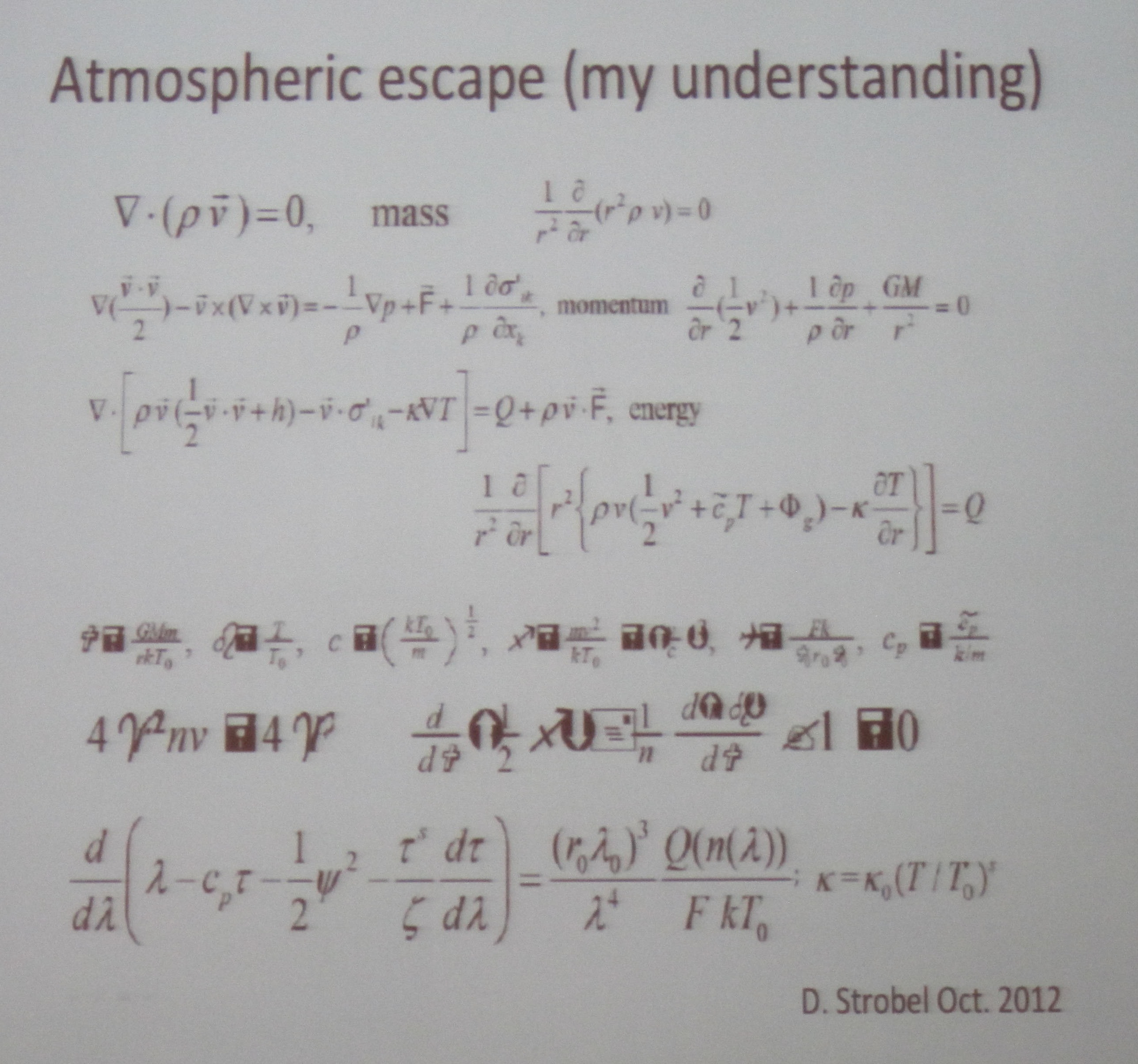
Yes, this is what an atmospheric modeler solves for. He/she solves numerous energy-balance, energy-transport, etc. equations to derive properties for making an atmosphere.

The Hydrodynamic escape rate is a key output from these numerical models for Pluto, with predictions in the range of 1.5-6.7 x 1027 particles/s. The basic problem with computing hydrodynamic escape is due to the presence of a gravity well that these molecules need to escape from. Essentially, you need an additional energy input (such as thermal) to drive the escape process.

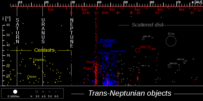
Some other key terminology: “The exosphere is a thin, atmosphere-like volume surrounding a planetary body where molecules are gravitationally bound to that body, but where the density is too low for them to behave as a gas by colliding with each other.” (Wikipedia) It is the uppermost layer where the atmosphere thins out and merges with interplanetary space. Theexobase is the lower boundary of the exosphere, defined as the altitude at which the atmosphere becomes collisionless.  Atmospheres can lose atoms from stratosphere, especially low-mass ones, because they exceed the escape velocity (Ve= (2GM/ R)½). This is known as (Jeans escape or Thermal Escape). The Jeans parameter (lambda) is a measure of how efficient the loss mechanism is. Larger lambda values implies less loss (smaller escape rates).

Models by different groups predict Pluto’s exobase between 5 and 10 Pluto radii. Assuming Pluto radius of 1200 km, Pluto’s exobase is in the 6000-12,000 km range. New Horizons’ nominal trajectory will bring the spacecraft to within ~10,000 km of Pluto’s surface and ignoring the slight fact that there are uncertainties in deriving Pluto’s size in the 20-100 km range and ignoring whether you determine a planet size by including or excluding the atmosphere, there is a possibility New Horizons could be flying through Pluto’s exosphere. Such an extended atmosphere could be affected by Charon and could affect Pluto’s interaction with the solar wind at the New Horizon encounter, as measured by New Horizons instruments PEPSSI and SWAP. (For more talk summaries about solar wind, see later blog entry).

A plot of temperature in Kelvin (x axis) vs. altitude in km (y axis) is a typical output of this type of model. Below is a particular plot shows the effect of adiabatic cooling, which Darrel Strobel stressed, is a key component that cannot be ignored. Another key output from these models is the computation of number density (N2 molecules/cm2/s) as a function of altitude.

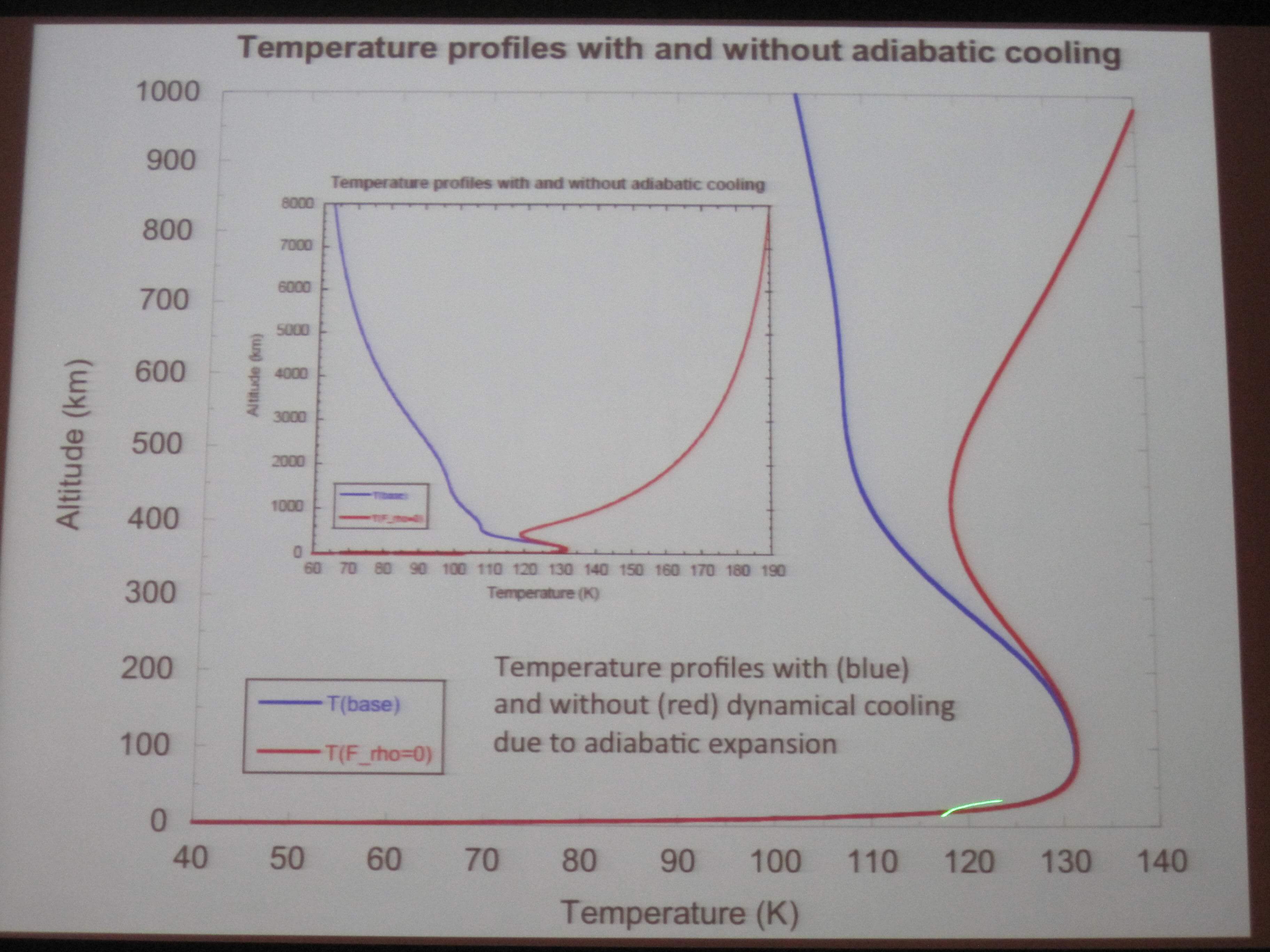
Temperature profile with altitude for models with (blue) and without (red) adiabatic cooling. The surface is at 40 K (which is from observation evidence) and upper atmosphere temperatures are in the 100s of Kelvin (supported by NIR spectral observations of methane). The two models predict wildly different temperatures at high altitudes depending on whether cooling is occurring.

Darrel Strobel’s predictions for New Horizons fly-by: Escape rate 3.5×1027 N2/s, exobase at 8 Rpluto ~9600 km, Jeans Parameter Lambda ~ 5.

Weather on Pluto. Fair, haze patches at first. Moderate calm with the occasional chop.

Reposted from https://blogs.nasa.gov/mission-ames/2013/07/24/weather-on-pluto-fair-haze-patches-at-first-moderate-calm-with-the-occasional-chop/.

The July 23, 2013 morning session of the Pluto Science Conference started with a collection of talks addressing what we know and what we don’t know about Pluto’s atmosphere.

Emmanuel Lellouch (Paris Observatory, France) spoke about “Pluto’s Atmosphere: Current Knowledge and Open Questions.”

What do we know about Pluto’s Atmosphere? We know that it is a nitrogen (N2) dominated atmosphere with methane (CH4) (tens of %) and probably carbon monoxide (CO). It’s about 10-microbar (pressure) class showing evidence for changes in pressure on year/decade timescales. There is also evidence for waves (dynamic changes), and the atmosphere does have a thermal structure, despite the details being hotly debated in the community (pun intended). People do agree that the surface is cold (40-50 K) and then the atmosphere is around 100K at micro-bar pressure levels. The details of the cold/warm layers in between are the stuff that thermal models are made of!

Pluto was discovered in 1930, but it was only in 1985 that the first observation detecting an atmosphere around Pluto was made. It was discovered through a measurement called a stellar occultation, when Pluto crossed between a star and an observer on Earth, on August 19, 1985 (Brosch, MNRAS, 1995). A higher signal-to-noise light curve was obtained on the June 9, 1988 (Elliot, et al 1989) occultation events whose light curves indicated existence of waves.

Occultation light curve for Pluto passing in front of a star on June 9, 1988 (signal vs. time) Features in this dataset indicate the upper atmosphere (above the ‘kink’) and lower atmosphere (below the ‘kink’). The ‘kink’ presence is theorized to be due to heating by methane (Hubbard et al 1990). Waves are indicated by the “spikes” in the light curve. When the scientists create this light curve from the occultation event, they then “invert” it to fit a temperature model and derive pressures for different scale heights.

The first molecular detection of anything in the Pluto’s atmosphere was methane (L. Young et al 1997) using the IRTF (3.5 m telescope) in May 1992. This was confirmed and re-measured in 2008 with higher resolutions and sensitivity (Lellouch et al 2009) using the VLT (8 meter telescope) with more recent observations in 2012. Emmanuel Lellouch showed that with those two latter datasets there was no evidence of change in the last four years. With this higher resolution data they can use it to provide a fit to the temperature using the line widths.

Carbon monoxide (CO) was detected in the submillimeter at 240 GHz with JCMT (Greaves et al 2011), but this detection and the inferred amount has lead to questions that the current models cannot produce this molecule with the temperature and amount inferred from the observations. This particular topic was addressed by Mark Gurwell’s talk later in the morning.

There is also evidence for diluted methane (CH4) and pure CH4 ice on Pluto’s surface. The atmosphere CH4 is much greater than what is expected from an ideal mixture, so this implies there must be a mechanism to enrich the CH4 component in Pluto’s atmosphere. Recent thermo-dynamic models and “GCMs” (general circulation models) predict a consistent mixture for CH4.

The combination of both the infrared spectral results and the visible (and in some case near-infrared) occultation light profiles helps resolve temperature profile (i.e., how temperature varies with altitude) inconsistences.

Speaking of temperature profiles, one of the hotly debated topics for Pluto atmosphere specialists is whether their models contain a tropopause. Per Emmanuel Lellouch’s overview talk, he stated, “There is no proof there is a troposphere. And deep troposphere are not predicted by the GCMs.” However, many Pluto atmosphere specialists often invoke a troposphere in their calculations to help predict other things that have been inferred to occur on Pluto.

Pluto’s atmosphere seems to be changing. There is observation of pressure evolution. Specifically, the pressure appears to have doubled from 1988 to 2002 (Sicardy et al 2003, Eliot et al 2003). Evidence that the pressure is continuing to increase is based on recent 2013 occultation data. This has led to the development of Volatile Transport Models. These are basically computations that track the dominant species, and for Pluto, it is nitrogen, through multiple temperature and pressure ranges, heat exchanges such as sublimation cooling in summer and condensation heating in winter. A schematic of a Volatile Transport Model from Leslie Young, New Horizons deputy Project Scientist, is shown below.

Schematic of a volatile transport model for Pluto. More details about the model are in a blog on Leslie Young’s volatile transport model talk later in the conference.

Other Oddities in Pluto’s Atmosphere. There appears to be evidence for photochemical haze from a 2002 occultation (Elliott et al 2003) but occultations in 2007 and 2011 did not show evidence of this. Hazes are large particles in the atmosphere (almost cloud-like) and the 2002 occultation had suggested hazes since there had been a distinct change in brightness as a function of wavelength. Why does the haze come and go, and what is causing it?

Pluto has also indicated “reddening” (color-change) that occurred between 2000 and 2002 (Marc Buie using color photometry with HST). That’s a mystery.

Waves (dynamic changes) in atmosphere are indicated by some of the occultation measurements. What could cause waves? There are multiple suggestions what could form these dynamic changes (even evoking the elusive gravity wave mechanism). Could it simply be Pluto’s atmosphere response due to the diurnal variation of sublimation of N2 particles?

What will Pluto’s Atmosphere be like when New Horizons comes to take a close look?

  • Will the atmosphere be there in 2015? Lellouch’s best guess: Yes.
  • Will there be a thermal structure (i.e. see a troposphere)? Lellouch’s best guess: Hopefully (helps modelers out).
  • Will there be other gases present (i.e. C2H2 HCN, etc.)? Lellouch’s best guess: Maybe.
  • Will there be clouds or hazes? Lellouch’s best guess: Maybe.
  • When will the atmosphere collapse (i.e. pressure drops by orders of magnitude)? Lellouch’s best guess: “Your guess is as good as mine.”

Comparative compositions of Pluto and friends, even long-distant friends.

Reposted from https://blogs.nasa.gov/mission-ames/2013/07/23/comparative-compositions-of-pluto-and-friends-even-long-distant-friends/.

Continuing coverage of the July 22, 2013 first day of the Pluto Science Conference being held this week in Laurel, MD.

Bill McKinnon (Washington University) next provided an engaging talk about implications for composition and structure for Pluto and Charon.

Where did Pluto Accrete (i.e. where was Pluto born)? Pluto is not alone in its location on that a/e plot for Trans-Neptunian Objects (see previous posting).  It’s part of an ensemble of bodies on the 2:3 resonance with Neptune, coined the group “Plutinos.” Was Pluto formed around 33 AU (Malhotra 1993, 1995) and then migrated outward? What does this Nice I Model (Levinson et al 2008) which migrates the giant planets predict for the KBO population? The Nice I Model implies that for Pluto, Pluto could have formed 20-29 AU (i.e. closer in) to allow it to achieve its high inclination. Then a subsequent model, Nice II (Levinson et al 2011), suggests Pluto may have formed in the 15-34 AU range. This is in okay-agreement with accretion models since Pluto, a 1000-km size body, would need 5-10 million years (i.e. within a nebular life) if it were formed in the 20-25 AU range. McKinnon’s best guess: Pluto formed between 15-30 AU.

How long did accretion take and what are the implications (i.e. how long for Pluto to grow up)? If we have an accretion time (10’s of million years), there is time enough to form Aluminum-26, which provides a form of heat through its decay. Heat then can melt ices and create a differentiated body (i.e., rocky core, icy mantle) and also drive water out. McKinnon’s best guess: Pluto formed rapidly and early.

What are Pluto & Charon made of? They are understood to be made of rock+metal, volatile ices, and organics, with rock+metal more than ice, and ice more than organics. The rock will be some combination of hydrated & anhydrous silicates, sulfides, oxides, carbonates, chondrules, CAIs (calcium-aluminum-rich inclusions), CHONPS (carbon, hydrogen, nitrogen, oxygen, phosphorus, and sulfur). We don’t really know what sort of composition these KBO volatile ices: will they be more like Jupiter Family Comets or Oort Comets? And we know even less about organic components: will the Nitrogen to Carbon ratio tell us whether KBO N2 (nitrogen) comes from organics rather than NH3 (ammonia)? Solar models (which lock up CO (carbon-monoxide) into carbon) can influence understanding of what rocks in the outer solar system are made of but their models are not in agreement with the best understanding of Pluto/Charon make-up. McKinnon’s best guess: Rock/Ice nature of Pluto-Charon is 70/30.

What are the implications for Pluto & Charon internal structure? New Horizons will not directly detect the differentiation state of Pluto & Charon because it does not fly close enough.

Alain Doressoundiram (Paris, France) came next. Using MIOSTYS, multi-fiber front-end to a fast EMCCD camera, on a 193 cm telescope in France, they observe outer solar system bodies using stellar occultations. Other science objectives for variable stars, transiting exoplanets. They confirmed two TNO occultation events, one in 2009 and one in 2012 and continue monitoring.

Luke Burkhart (Johns Hopkins University) talked about his work on a “Non-linear satellite search around Haumea.” Haumea is another Trans-Neptunian Object (TNO) that has multiple satellite companion, like Pluto. Using HST (10 orbits) they observed the Haumea system and used a method of stacking & shifting to identify satellites. But this method fails to capture objects which are close in, moving fast, and on highly curved orbits. So they developed a new method using a non-linear shift-rate. Their approach, when applied to the Haumea system, had a null-result. However, this approach could be used on images of the Pluto system and other TNOs.  Specifically, in answer to a question from the audience, Luke would be eager to use his technique on any of those long-range KBO targets the New Horizons project is currently investigating.

eighttnos

Family portraits of the eight largest trans-Neptunian objects (TNOs) (From http://en.wikipedia.org/wiki/Trans-Neptunian_object). Pluto is shown with its 5 companions.

Andy Rivkin (JHU/APL) ended the afternoon’s lively discussion by addressingDistant Cousins: What the Asteroids Can Teach us About the Pluto System”. He started his talk with a comparison of sizes between Ceres (the largest asteroid in the asteroid belt between Mars and Jupiter) and the Pluto System. He used as his framework Emily Lakdawalla’s chart, which can be found on the Planetary Society blog http://www.planetary.org/multimedia/space-images/charts/relative-sizes-pluto-system.html.

Here the relative sizes of objects in the Pluto system are represented by objects from the Saturn system. Saturn’s moon Rhea serves as Pluto, Dione as Charon, Prometheus as Nix, Pandora as Hydra, Helene as Kerberos, and Telesto as Styx. Superimposed is where Ceres (an asteroid in our asteroid belt between Jupiter & Mars) fits on this scale. Andy Rivkin did a comparison of his observations of Ceres to postulate what that might mean for the Pluto system.

Pluto system and Ceres shown to scale, represented by objects from the Saturn system.

Ceres has an icy interior, but much too warm to keep ice on surface. HST images reveals rather smooth surface. IR spectra (from reflected sunlight) are very rich and indicative of ice-type features. Could there some sort of layering? On Pluto, you could have the same thing, but it’s also cold enough for ice to remain on the surface. There is also a mystery that several large C asteroids have similar 3 micron spectra to Ceres like 10 Hygiea and 704 Interamnia.

Implications for Pluto: Large main-belt asteroids could serve as comparisons for KBOs. Geophysical comparisons may be easier than compositional ones.

So the big take-away from the introductory talks on the “Kuiper Belt Context” is that we can learn more by sharing the knowledge: Learning from Other Bodies  (Other TNOs, Comets, Asteroids) will help us learn more about Pluto & Charon, and vice versa.

Finding that distant KBO needle in a deep space haystack.

Reposted from https://blogs.nasa.gov/mission-ames/2013/07/23/finding-that-distant-kbo-needle-in-a-deep-space-haystack/.

Next up at the Pluto Science Conference were a series of talks dedicated to recent work in the searches for another Kuiper Belt Object (KBO) for the New Horizons spacecraft to fly by after its Pluto fly-by. Fuel on board the New Horizons spacecraft after the July 2015 Pluto fly-by could enable a fly-by of a distant KBO in the late 2010s through 2020s, pending identification of targets reachable within New Horizon’s remaining fuel budget.

John Spencer (SwRI) has been leading the ground based campaign to search for New Horizons’ next target. With an on board ~0.13 km/s delta-v (measure of propellant), traveling at 14 km/s, this translated to a ~0.5 deg half-angle cone through the Kuiper Belt for accessible targets, a type of “survey beam.” Previous KBO searches had been for R>26.0 over 1-2 degrees. But right now Pluto is in Sagittarius which is in the direction of the Galactic Center and there are a lot of other stars in the field that make searching for a slowly-moving object, this KBO, difficult.

img_1135

Above are what the star fields the team is inspecting look like. They observe the same star field night after night and look for shifts in a object between frames, indicating it’s a KBO and not one of the “fixed stars.”

611px-outersolarsystem_objectpositions_labels_comp

“Known objects in the Kuiper belt, derived from data from the Minor Planet Center. The pronounced gap at the bottom is due to difficulties in detection against the background of the plane of the Milky Way.” This is exactly where John Spencer and his team are focusing their efforts because a subsection of that part of the sky is what is reachable by the New Horizons spacecraft after 2015. Image taken from http://en.wikipedia.org/wiki/Kuiper_belt.

The ground based search program area is entering a sweet spot, where they can cover a smaller area of sky from the Earth that falls within the expected New Horizons travel zone.

The team has found 31 objects from 2011 data including a TNO. However, as of 2012 season, they have not found an object that could have a fly-by encounter by the New Horizons spacecraft.  But there are three objects (2011 JW31, 2011 JY31, 2011 HZ102) that New Horizons could get to within 0.15-0.2 AU of in 2018-2019. The team is in the middle of the 2013 observing season and based on the current number densities they are predicting to see 1.78 objects down to  R=26.0mag and 4.15 objects in 26.5 mag.

Alex Parker (one more month at Harvard before moving to Berkeley) provided a more in depth view of unique observations New Horizons can still make of these long-distance KBO fly-by, that is, a fly-by in the 0.1-0.2 AU range of the spacecraft. At 0.2 AU range, New Horizons’ LORRI will have 140 km/pixel range compared to our “sharpest eyes” by Hubble at 1200 km /pixel from low-Earth orbit.

His excitement over the unique discovery space New Horizons provides that you cannot get from anywhere else: Proximity. High angular resolution. High phase angles.

He’s been studying trans-Neptunian binaries as binaries provide a direct mechanism to measure their masses. “Wide” Kuiper Belt binaries have been discovered already (e.g.  Gemini observations of wide binaries 2006 BR284 separated by 0.82 arcseconds; 2000 CF105 separated by 0.95 arcseconds).

To visualize a ride on looking over the New Horizons shoulders as it journeys into the Kuiper belt, check out this one of Alex Parker’s visualizations at Vimeo.com/alexhp/newhorizons.

Make note to hold onto your seat when the craft enters the Cold Kuiper Belt region in 2018!

Susan Benecchi (Carnegie Institute) rounded out the talks with HST Follow-Up Observations of Long-Range Candidates for New Horizons post Pluto. They observed 2011 JW31, 2011 JY31, and 2011 HZ102 with HST. Those objects had been detected with the KBO ground based search program described by John Spencer and Alex Parker (previous presentations). Her team has not confirmed detection of 2011 JW31. Her team has confirmed the colors of the two other objects being “red” which is consistent with the Cold Classical Population (i.e. primordial). Implications for New Horizons: HST can provide this extra characterization step for new candidates.

Gustavo Beneditti-Rossi (Brazil) described a summary of “Astrometric Analysis of 15 years of Pluto Observations.” Using the Pico dos Dias Observatory (1.6m and 0.6m telescopes), they monitored Pluto-Charon (which is not separated in their data) for 154 nights over 1995 to 2012. They do refraction correction (due to viewing angle from earth) and photo-center correction (due to the fact they cannot separate Pluto from Charon). And show that their tracking of Pluto’s location is in agreement with occultation data.

To end this post, I could not resist showing you Alex Parker’s vision of what New Horizons brings to this field of study. He created this montage of images illustrating the proximity (within artistic license) and equally important the high phase (objects as crescents) and high angular resolution (we can see surface features), all that New Horizons will provide in 2015 that no other observation platform can.

parker_nh_montage

2015 will be the “Year of Pluto” and so much more!

Pluto, “King of the Kuiper Belt, Prince of the Plutinos.” Certainly an object that inspires odes, songs, and ballads.

Reposted from https://blogs.nasa.gov/mission-ames/2013/07/23/pluto-king-of-the-kuiper-belt-prince-of-the-plutinos-certainly-an-object-that-inspires-odes-songs-and-ballads/.

After the New Horizons’ instrument overviews on the first day at the Pluto Science Conference (Jul 22, 2013, we jumped right into Pluto in the Kuiper Belt Context.

Brett Gladman (University of British Columbia, Vancouver, Canada) started the conversation by addressing “How does Pluto fit in our understanding of the Kuiper Belt?”

But before we get into that, discussing the Kuiper belt today can be pretty complex. It was only discovered in 1992, but in the years since, over 130,000 bodies with sizes 100 km and larger have been identified (Petit et al 2011), with Pluto being the largest member.

So when we start looking at large numbers of objects, it’s time to classify. So a typical plot to describe these “populations” is shown below, where semi-major axis (distance of body from the Sun) is plotted (horizontal axis, labeled ‘a’ in units AU, where 1 AU is the distance of the Earth from the Sun, Jupiter is ~5 AU, Saturn ~10AU) versus eccentricity (value between 0 and 1 that describes how circular an orbit it, e=0 is circle, e=1 is parabola, 0<e<1 describes ovals).

And then you have your Classical, your Cold Classical, Hot Classical, Detached, Resonant, and SDO (aka Scattered Disk Objects), etc. Sometimes they group together, others are more uniform across the parameter space.

Kuiper Belt in “a/e space.” Cold classical (black open triangles). Resonant Kuiper (open red square). Detached (blue triangles). Pluto is indicated with the yellow-box, it’s a Resonant, as it is in 3:2 Resonance with Neptune. This group of objects, all in 3:2 Resonance with Neptune are the “Plutinos.” (that clumping around 40 AU, red triangles, spanning over a range of e). Resonance numbers are shown at the top of the graph.

Plutinos are also a family of TNOs, Trans-Neptunian Objects, characterized by being in 3:2 mean-motion resonance with Neptune (i.e., every time Neptune makes 3 trips about the Sun, the Plutinos make 2 trips). Plutinos are the most dominant of the TNOs. Less numerous are the 1:1 objects, objects known as Trojans.

Definitely KBO soup!

For more information about TNOs and their period relationships with Neptune https://en.wikipedia.org/wiki/Resonant_trans-Neptunian_object.

After getting down those nomenclature basics, Brett Gladman (who is also lead for a huge ground-based survey of KBOs called the Canada-France Ecliptic Plane Survey/CFEPS) discussed the strengths and pitfalls of the theories put forward to explain the formation and structure of this complex KBO menagerie.

For more information about CFEPS check out http://www.cfeps.net/.

How did Pluto get to where it is today? Two leading theories (1) Resonant sweeping of objects formed in TNO regions and (2) resonant trapping explain many things, but no published models explain those resonant structures of the Kuiper belt. And any of these models have issues with the classical and scattering disk populations as well. Theorists, better sharpen your pencils.

So he left us with questions to ponder. Is there a cold primordial Kuiper Belt with edge at 45 AU? Did Pluto likely form as one of hundreds to thousands of >1000km embryos? Did some of these become implanted into the nearby non-scattering belt? Are there others out beyond 100 AU (considered likely, but to discover them, you need to get down to 23-24th mag which is beyond the current survey capabilities until new telescopes and.or techniques come available)?

No doubt, searches for more TNOs will continue, the classification of the KB will undergo evolution, and theorists will refine their models. And New Horizons will provide a unique data set of an up-close-and-personal visit to Pluto and its companions to help constrain those models.

800px-thetransneptunians_73au-svg

Putting Centaurs and TNOs in Context. This time plotting inclination (the degrees from the ecliptic plane) vs. semi-major axis in AU. Object sizes are reflected in the symbol sizes. Location of Saturn, Uranus and Neptune are shown. Just another way to look at that awesome & diverse Outer Solar System. From: https://en.wikipedia.org/wiki/Trans-Neptunian_object.

Next, Cesar Fuentes (Arizona State) phoned in about his work on the “Size Distribution (SD) of the Kuiper Belt.” Size distribution is basically counting the number of objects as a function of size.  Coagulation (of small particles) and gravitation instability (of larger particles) shape the size distribution. Size distribution is expected to change due to collisions. Different distances from the sun also appear to have different size distributions.

He stepped us through recent size distribution models from Schlichting, Fuentes & Trilling (2013) and Kenyon & Bromley (2013) where they even have some including the “collisional factor” influence on the size distribution over time periods.

All the Size Distributions show a “rollover” around H~9, D=70km. Nesvorny et al. 2013 investigates this further. Is the break due to collisional and therefore separate the primordial from the evolved KBO populations?

Even more questions to ponder:  Can we use size distributions to evaluate primordial from the evolved KBO populations?

And then he left us with a tantalizing experiment with the New Horizons mission: If New Horizons can provide data sets enabling “crater counting,” we will be able to measure the impactors on Pluto. This can aid in understanding KBO populations, addressing specifically, formation time, timescales for surface activity, and origins of bodies like Nix & Hydra. What would a 0.1-100 km impactor size distribution look like?

Pluto, be it Prince of the Plutinos or King of the Kuiper Belt, will always remain a key part to these questions above. And data sets from New Horizons will provide many new angles to answering questions about “Where did Pluto form and why did it wind up where it is now.”