Tag Archives: New Horizons

Coordinate systems do matter. Brush up on that Right Hand Rule, y’all.

Reposted from https://blogs.nasa.gov/mission-ames/2013/07/26/coordinate-systems-do-matter-brush-up-on-that-right-hand-rule-yall/.

This is a blog series covering the talks presented at the Pluto Science Conference, held July 22-26, 2013 in Laurel, MD.

In an engaging talk by Amanda Zangari (SwRI) entitled “Plutography: A Meta-Analysis of Coordinates on Pluto From Charon’s Discovery to the Present Day,” she compared and contrasted two coordinate systems used by Pluto researchers. Her motivation is that data sets, past, present and future will be compared to the New Horizons dataset, and so it will be very important that all use the same coordinate system.

coord_conv_1

It comes down to two coordinate systems, although she mentioned that some researchers sometimes use a hybrid-definition.  In her visual summary, the Red (left) is the Ecliptic North configuration where Pluto’s North Pole is “North of the invariable plane.” The Green (right) is the where “Pluto’s North Follows the Angular Momentum Vector” aka Right Hand Rule (RHR).  When the planet’s north pole is aligned closely with the Ecliptic North, the former is normally okay (like for Earth). However, for Pluto, Uranus and Venus the two are definitely very different. She suggests that the Right Hand Rule is the more appropriate definition for Pluto. Note that JPL Horizons (their official ephemeris generating software), GEOVIZ (New Horizons Planning software) and SPICE uses the other convention (Ecliptic North Pole).

How they differ are summarized below (i.e. both axes are flipped). The pole that is visible from Earth is what is seen in the lower-right quadrant of each schematic. Since the 1980s we have been is observing Pluto’s Northern Pole per the Right-Hand-Rule (RHR) convention.

coord_conv_2

Alan Stern, New Horizon’s Principal Investigator (lead scientist) mentioned that the New Horizons Spacecraft will not change its system prior to the Jul 2015 encounter. After the encounter, the plan will be to adopt the new SPICE files, etc. He stressed that Pluto Data that gets released in the Planetary Data System will be in the Right-Hand-Rule convention (RHR). Leslie Young, New Horizons’ deputy Project Scientist, said that there are new SPICE files available using a Pluto coordinate system using the RHR Convention, although the JPL/SPICE official release  is still Ecliptic North.

So, huh, which way is up? I’m sure this topic is far from over. In fact, during discussions at the meeting, agreeing on a coordinate system for planetary bodies is no stranger to this community.

Did you know it’s northern springtime on Pluto right now? Pluto is far from a cold lump of rock we were told about in school. It’s a dynamic world and has seasons.

Reposted from https://blogs.nasa.gov/mission-ames/2013/07/26/did-you-know-its-northern-springtime-on-pluto-right-now-pluto-is-far-from-a-cold-lump-of-rock-we-were-told-about-in-school-its-a-dynamic-world-and-has-seasons/.

The afternoon session of Jul 25th of the Pluto Science Conference started with John Stansberry’s (STScI) talk entitled “Interactions between Pluto’s Surface and Atmosphere.” He stated, “The similarities between Pluto and Triton are remarkable.”

The main properties of Pluto and Neptune’s moon Triton are summarized above.

Pluto has a volatile-rich atmosphere (N2, CO, CH4) and interacts with the surface to bring about mass and energy exchange. N2 dominates the surface ices and the atmosphere. N2 is also globally much at the same temperature mainly due to N2’s large latent heat of sublimation that balances out changes in temperature. To probe deeper at surface-atmosphere interactions, he looked specifically at the methane to nitrogen mixing ratio (abundance of one component of a mixture relative to that of all other components). But there are many open mysteries about surface-atmosphere interactions.

Overabundance of Methane Mystery.  Pluto’s upper atmosphere has X_CH4 ~0.5% (X_CH4 is the methane mixing ratio) based on occultation measurements. Infrared spectral measurements (Jason Cook et al 2007) from the lower atmosphere derive a much higher X_CH4 ~ 4%. Surfaces models for the N2+CH4 ice predict  X_CH4 ~0.5%. So in order to explain the overabundance of methane in Pluto’s lower atmosphere, two models were introduced to help provide additional sources of methane. This is an active area of study.

Changing Atmospheric Structure. Stepping through the light curve changes shown by Mike Pearson (see previous blog entry) there is something changing the structure of the atmosphere at ~1200 km. Comparing 1988 (equinox) and 2006 (N mid-Spring; Northern ) could be explained partially by geometry changes. Not all the changes are understood.

Pluto’s lower atmosphere is a mystery. We can probe down to the stratosphere with occultation measurements (scale height 50 km). So below 50km they need to resort to models.

Other influences on surface-atmosphere interaction included effects due to topography and winds. Winds have been observed on Triton (Hansen et al 1990).

Predictions for New Horizons. X_CH4 will be ~0.5% in stratosphere, a few % in troposphere. For the atmosphere structure he predicts r_tropopause = 1185 km, h_tropopause = 10km, r_atmosphere_base = 1200km, weak inversion, and bottom of atmosphere at r=1175 km, pressure at surface > 15 microbar. Winds will be Triton-like. A bright north polar cap. Potentially morning frosts.

Bonnie Buratti (JPL) presented a talk on “Pluto’s Light Curve over Time as an Indication of Seasonal Volatile Transport.” They are looking at historical light curves, plus new ones and fit with a fixed frost model. Changes in light curves tell you about the albedo (reflectance) of the surface. You do need to do a correction to phase angle because of Pluto’s high obliquity. They do find the data over 2012-2013 consistent with a constant frost model. She showed the data of long-term monitoring of Triton and it indicated a volatile change and they got HST imaging data which when compared with the Voyager fly-by they did see that areas of high albedo got dark and others got brighter, supporting their interpretation of the light curve approach. They really need to get a good light curve prior to New Horizons’ 2015 fly-by encounter.

Erin George (University of Colorado), working with Marc Buie (SwRI) in “Pluto Light Curve in 2010,” described her work in analyzing data from Lowell Observatory over 2007-2013. The challenge had been to find stars to use as relative flux calibrators that were well separated. They also used a technique to remove the template of background stars (eliminate field confusion).

Marc Buie (SwRI) next took us on a tour of “Seasonal Variations on the Surface of Pluto.” He reports on visible (B & V filters)  photometry from data taken with photographic plate, photoelectric detectors, and CCDs from 1954-2010. All the measurements are of “Pluto+Charon” as the two bodies are not resolved from the ground for the majority of this data (large pixels). He showed the trend of the light curve which indicates that “something happened in 1992” (he hypothesizes it occurred very fast) to change the “color” of Pluto because the light curves in B & V passbands deviate. He’s working towards removing Charon from the data using a model for its brightness from his HST data.

Leslie Young (SwRI) presented a talk on “Modeling Pluto’s Diurnal and Seasonal 3-Dimensional Volatile Transport with VT3D. ” She asks, “Why should we care about volatile transport?” Three key reasons: (1) Mobile volatiles control the surface appearance (albedo, composition), (2) Volatile transport depends on the hidden subsurface (thermal properties, depth of volatile deposits), and (3) Volatile transport models can predict atmospheric behavior at other times (escape rates, atmospheric chemistry, winds).

Her new code, VT3D, uses physics from standard volatile transport models (Hansen &  Paige, Spencer & Moore). She has been validating it against other codes. Types of parameters that she investigated in her code are emissivities, thermal inertia, albedo, and nitrogen abundances. She found her results clumped into three categories, atmospheres characterized by: (1) Permanent Northern Volatiles, (2) Exchange with Pressure Plateau, and (3) Exchange with Early Collapse.

A description of her model can be found in L. Young (2013) http://arxiv.org/abs/1210.7778.

Her model fails to predict a bright south pole seen in the 1990-1994. But then she counters, could that be possible because it’s covered with bright CH4 frost?

Three classes of atmosphere models from Leslie Young (2013). The graphs are the surface albedo and the pressure at  1175km in u=microbars vs. time. The time runs from 1866 to 2116, a full Pluto year about the Sun. The seasons on Pluto are shown with the vertical lines and the equinox in 1990 is highlight with the circle.

To learn more about Pluto’s seasons check out this blog from the Planetary Society http://www.planetary.org/blogs/emily-lakdawalla/2013/05021212-plutos-seasons-new-horizons.html.

Candy Hansen (PSI) described her model in her talk entitled “Pluto’s Climate Modeled with  New Observational Constraints.” She described her model, HP96, named after Candy Hansen and her collaborator Dave Paige, which was coded in 1996. She showed an output of the model for Pluto from 1000 to 2100 AD, over a good four Pluto-orbits about the sun. The model now has been updated to address new knowledge learned about the Pluto system.  To derive solutions that do not have a zonal band (an observable characterized by sharing a range of latitude, appearing as a ‘band’), eliminates high thermal inertia cases, cold frosts and large abundances of N2. The model does meet constraints from the observed albedo. She does not include an atmosphere in her model, so she is excluding wind and other atmosphere layer issues. After seeing the data from the May 2013 occultation presented at this meeting on Tuesday made her change her models and she presented a true “hot off the press” new result today. Predictions for New Horizons. 2.4 Pascals at the surface at the time of the New Horizons fly-by.

As a closing comment during the discussion session, Rick Binzel is hopeful that Charon-illuminated image of Pluto’s south pole during the New Horizons fly by will be a key to helping understand what may be going on at Pluto’s south pole!

A nice summary of seasons of Pluto. Since the 1950s we are seeing more of Pluto’s northern hemisphere. We are in Pluto’s northern spring time right now.

Laurence Trafton (University of Texas) gave a talk on  “Driving Seasonal Sublimation and Deposition on Pluto-Uncertainties in Evaluating the Vapor Pressure.”  Pluto’s atmosphere is supported by the vapor pressure of its surface ice.  For most models, N2, CH4, and CO are assumed to exist solely in solid solution on Pluto’s surface, and are well mixed in atmosphere. However, this did not explain the mystery of Pluto’s elevated atmosphere CH4 amounts (seeabove talk by Stansberry). Two models were suggested: “Detailed balancing model” (DBM) (Trafton 1990) and the “Hot CH4 Patch Model” (Stansberry et al 1996).  The latter only needs 1-3% of Pluto’s surface to have this extra source of CH4. Neither model can explain widespread pure CH4 ice hypothesized to be on Pluto’s surface. He is in need of lab experiments to establish vapor pressures for the saturated areas of the phase diagram.

Tim Michaels (SETI) spoke about “Global Surface Atmosphere Interactions on Pluto. ” He is using the OLAM (Ocean Land Atmosphere Model, Wakko and Avissar, 2008) model. He is using the Northern summer in 21st century convention (which is the IAU/Ecliptic North coordinate system). Their approach stats with a simple surface nitrogen ice model (no methane). When run for 1990 and 2015, they show distinctly different trends. Next steps are to add albedo distribution, methane cycle, and gravity changes. This is a rich atmosphere-surface system.

Kevin Baines (University of Wisconsin-Madison) spoke about “Chemistry in Pluto’s Atmosphere and Surface: Predictions of Trace Aerosol and Surface Composition, and a Potential Geologic Chronometer.” There are many sources that drive atmosphere surface chemistry and albedo. For example, volatile transport dominates on days, months, and year timescales. There is UV photochemistry (decade timescale) in this rich atmosphere. Hydrocarbons could be raining out 1mm every 50,000 years. Solar wind and accretion activities (impacts, dust from satellites or KBOs) occur in 1Myr timescales. So, he asked, “What would Galactic Cosmic Rays(GCR) do?“ The types of products by irradiation from CGRs include CH4, CnH2n+2, C6H10, NH3, HCN, etc. over 5-20 Myr. And he proposes they may be viewable by darkening on airless KBOs.

Vladimir Krasnopolsky spoke on “Pluto’s Photochemistry:  Comparison with Titan and Triton.” There are three bodies with N2/CH4 atmospheres in the solar system: Titan (moon of Saturn), Triton (moon of Neptune), and Pluto. He proposes that Titan is a better analog to Pluto rather than Triton. He presented the main results of his Pluto Model (Krasnopolsky & Cruikshank 1999). He observed Pluto with HST in the UV 180-256nm and was able to fit molecular species predicted by his model and saw no albedo changes from his predictions (Krasnopolsky 2001). New Horizons data will provide useful information to update their photochemical model.

Francois Forget (CNRS, Paris, France) closed the day with “3D Modeling of the Methane Cycle on Pluto). He presented the LMD Pluto Global climate model. Their model does include the methane cycle, but they are neglecting microphysics of N2-CH4. They assume the terrain description of Pluto from Lellouch et al 2000 (areas of N2 Ice, CH4-rich areas and dark albedo areas due to tholins). They ran the model starting from 1988 and the model has a resolution of 170km. The model predicts an observable X_CH4 of 0.35% and this in the agreement of the ~0.5% from observational data by Lellouch et al (2011). The models predict methane cloud formation at the pole and that could be matching observed data from J. Cook who understanding his methane detection comes form cold parts of the atmosphere. He presented a model for cloud formation for 2015 and clouds do appear in the low, colder parts of the atmosphere. Their model will be made available to the community to use. They do not have a cold troposphere in their model.

Prediction for New Horizons. More CH4 ice deposits at the summer pole in 2015 than in 2010.

Who’d have known that that little cold world out there in deep, dark space, would have such a fascinating trip around the Sun? Data from New Horizons from its July 2015 fly-by of the Pluto System will literally confirm or refute all of these predictions. Then the models can be updated to reflect what summer will be like on Pluto in 2240.


Today: Geology of unmapped worlds. 2015: Pluto will never be the same as New Horizons brings you a Pluto, Charon, Nix, Hydra, Kerberos, and Styx, in ways never seen before.

Reposted from https://blogs.nasa.gov/mission-ames/2013/07/26/today-geology-of-unmapped-worlds-2015-pluto-will-never-be-the-same-as-new-horizons-brings-you-a-pluto-charon-nix-hydra-kerberos-and-styx-in-ways-never-seen-before/.

This a blog entry for a series about the Pluto Science Conference being held at JHU’s APL in Laurel, MD, July 22-26, 2013. This entry summaries surface geology talks presented on July 25th.

Paul Schenk (LPI) began the session with his talk entitled “The Improbable Art of Predicting Pluto-Charon Geology.” Thanks to Voyager, Galileo and Cassini we have a wealth of knowledge about icy bodies in the solar system. However, in comparison to the icy satellites about Saturn, the Pluto-Charon bodies are expected to have key differences: volatile ice content is probably higher, their geological histories are not influenced by the existence of large giant planet near by (tidal forces), etc.

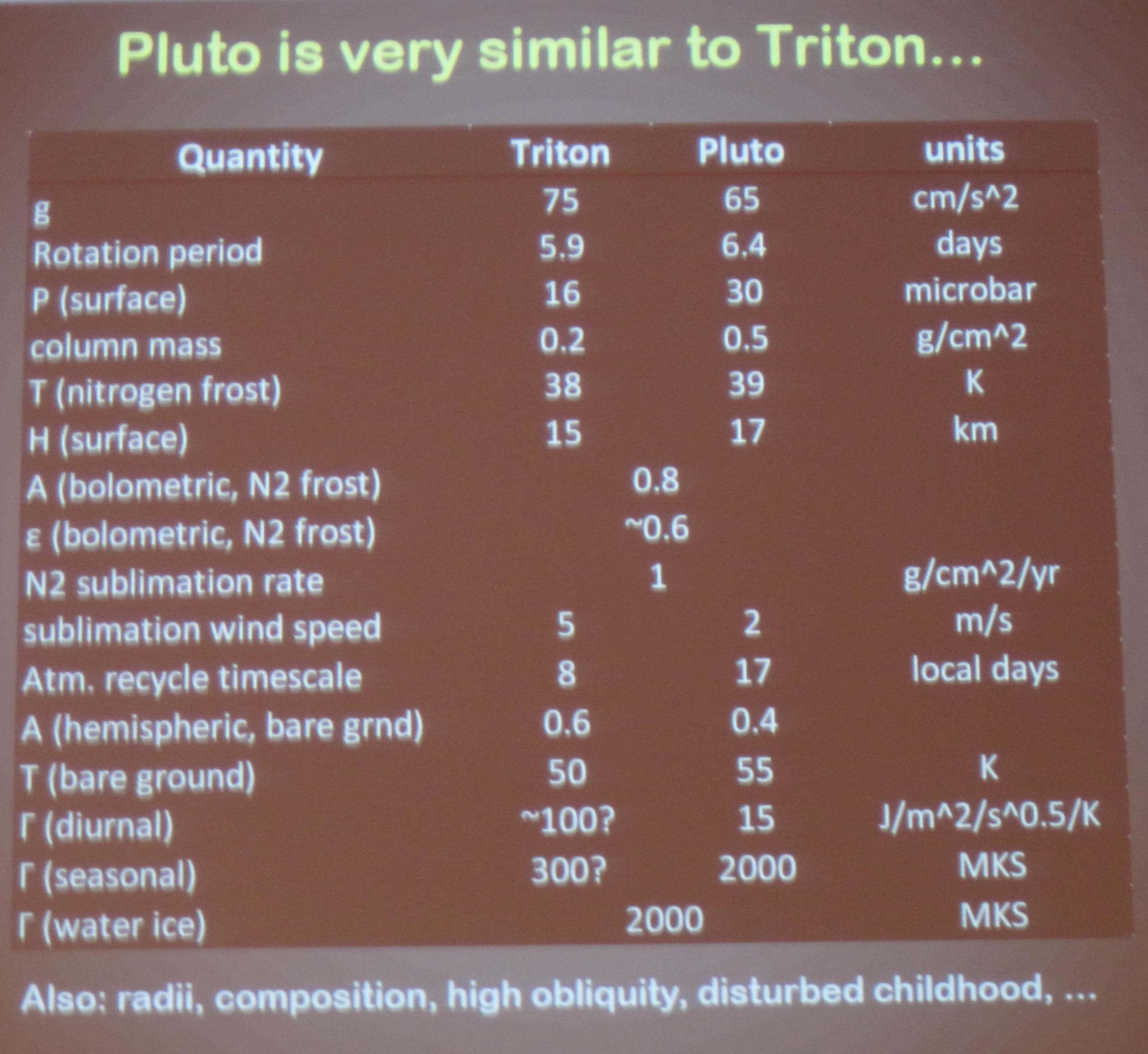
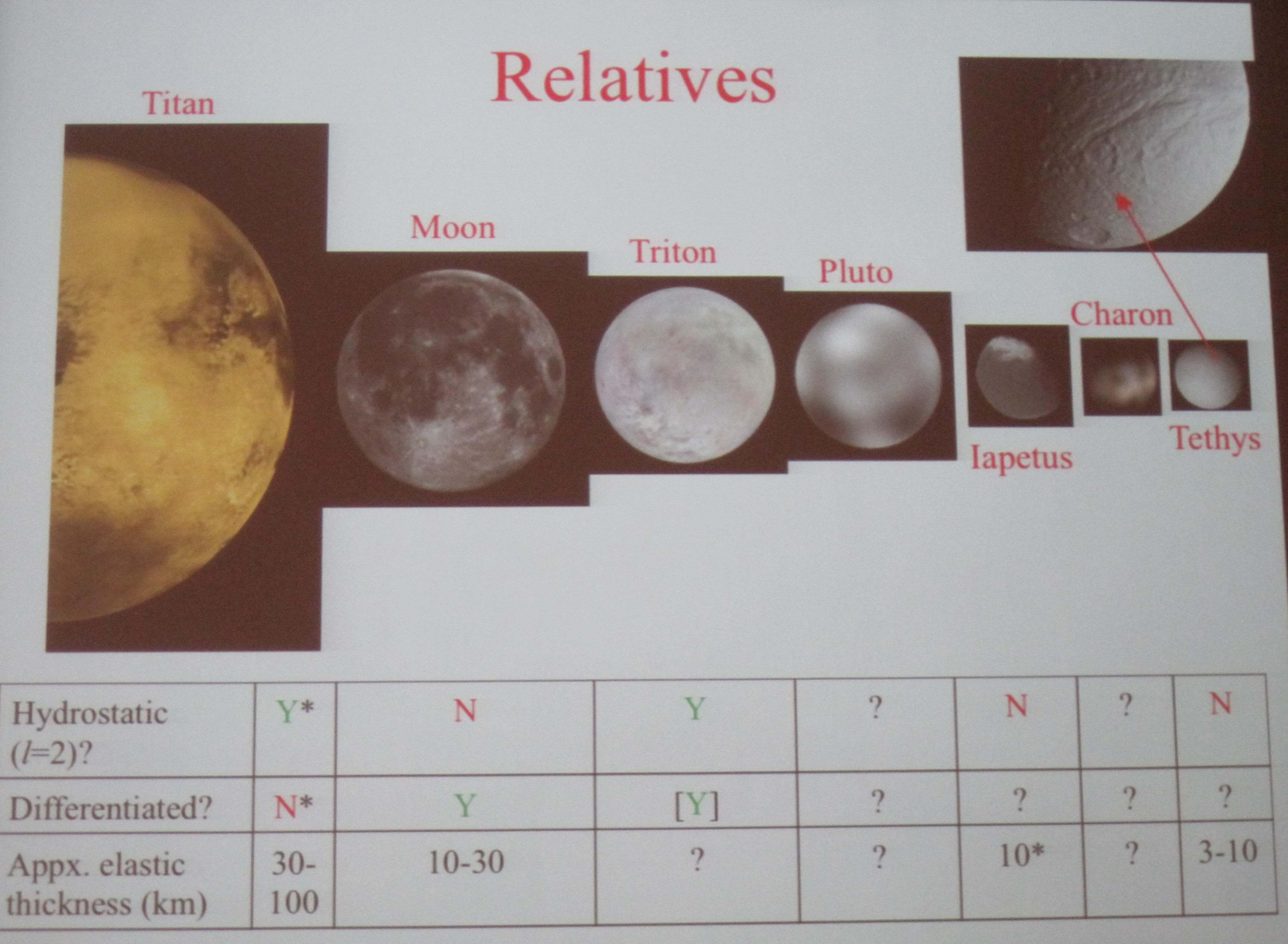
He asked, Is Pluto just another Triton? No. It may be similar in size and composition, but geology will be different. The main sources for heating for Pluto are assumed to be heating from radiogenic rock component (heating by radioactive decay) and energy from the giant impact that formed it. Is Charon one of many? Charon is of similar size to Uranian satellites Dione, Tethys, Ariel, Umbriel, but it may be that Charon-forming impact did not much impact much heating. In any event, all these icy satellites are diverse, from dead cold worlds to those with active erupting volcanoes, so in Paul Schenk’s words, “Who knows [what Charon will resemble]?”

He next stepped up through the key geological processes that would alter and/or create surface features. For example, volcanism creates smooth plains, calderas, vents, ridges, and active venting. Volcanic processes have been seen on many icy moons. There is diapirisim, a type of solid-state resurfacing due vertical ice movement. To have this process, you need an ice shell, preferably a thin shell with a source of heat. This is seen only two icy bodies in the solar system: Triton (“cantaloupe terrain”) and Europa (domes, spots). There is also tectonism, revealed through fractures.

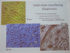
Vertical movement is one of the processes creating unique features on Triton & Europa. The Earth shows this behavior (described above, called diapirism) in local regions of salt deposits.

He next pointed out the possibility that satellites could have rings too. For example, there is a giant ridge on Iapetus (Ip 2007) and a similar feature on Rhea (Schenk et al 2011). It is hypothesized that these surface features were the result of a ring that had collapsed onto the surface. His advice to the New Horizons team is to pay special attention to the Pluto-Charon equatorial regions to look for a ring-remnant.

Impact Cratering tells us about the impactor population that are “fluxing into the system,” reveals surface stratigraphy, reveals interior stratigraphy (what the underlying layers look like), and reveal thermal history. Counting crater impacts on Pluto & Charon will be used to evaluate the Kuiper Belt population.

Predictions for New Horizons. He expects craters to look like those found on Ganymede (simple craters) for Pluto and Dione & Thetys for Charon (craters with dominant peaks). Charon may be “bland geologically.”

What about viscous relaxed craters? They have been found on Ganymede & Enceladus. Crater shapes can be used to reveal the properties about the object. However, he added this caveat that all previous work on modeling crater shapes was on water ice dominated surfaces, not methane (which is expected on Pluto), so more lab work is needed. Basin morphologies are important too. They tell us about evolution. Anomalous morphologies are also a key thing to look for on Pluto & Charon.

europa_tyre

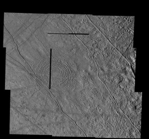
The Tyre crater on Europa (one of Jupiter’s moons) fromhttp://www.lpi.usra.edu/science/kiefer/Education/SSRG2-Craters/europa_tyre.jpg.

Europa has these intriguing multi-ring systems, such as shown above with the image of Tyre crater. The hypothesis is that on Europa we are seeing an impact penetrating into the ice shell of 10-20 km. Crater falls in on its self, creating this ringed structure.

“There will be impact craters. We are going to be captivated. We are going to be befuddled.” – Paul Schenk

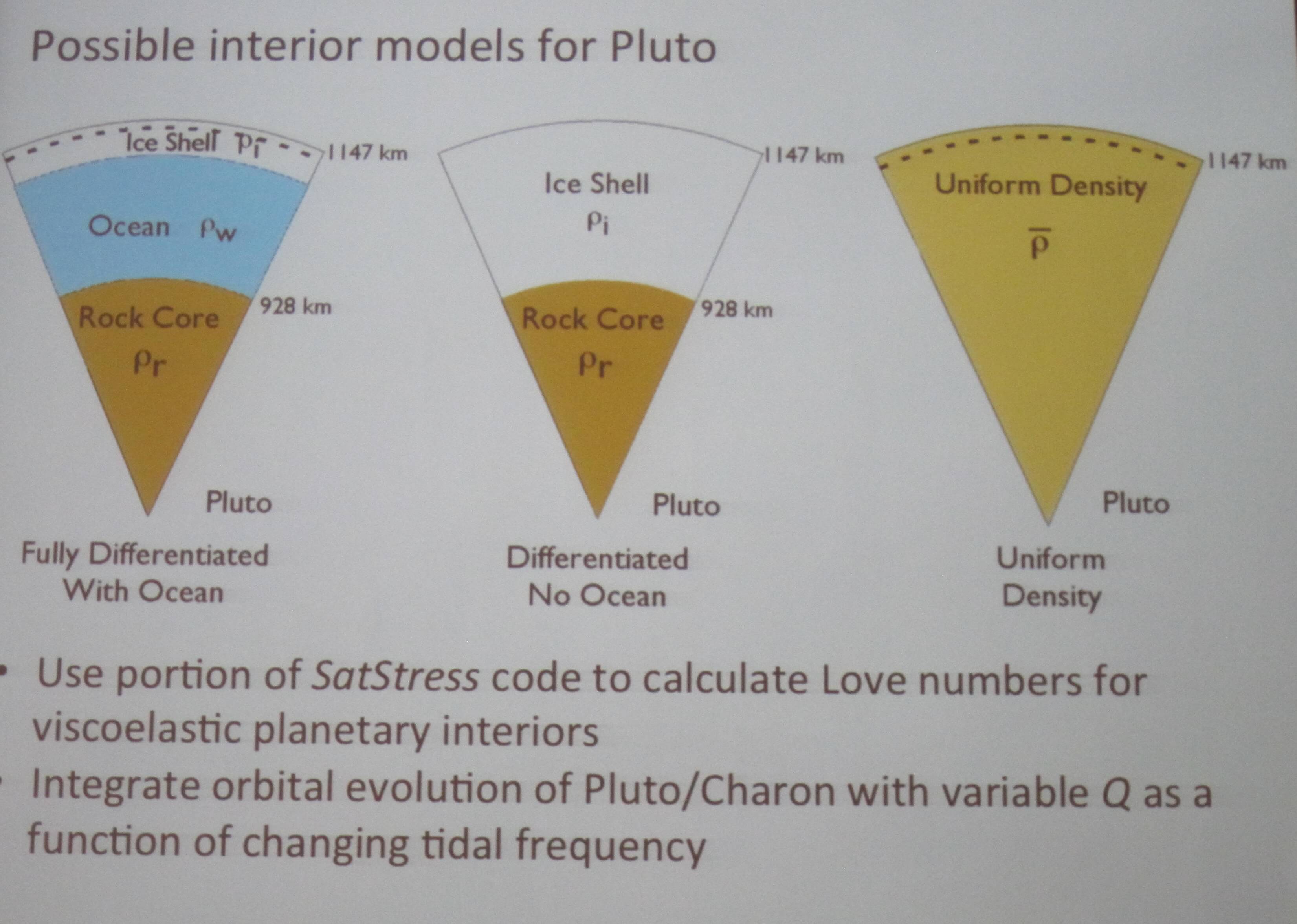
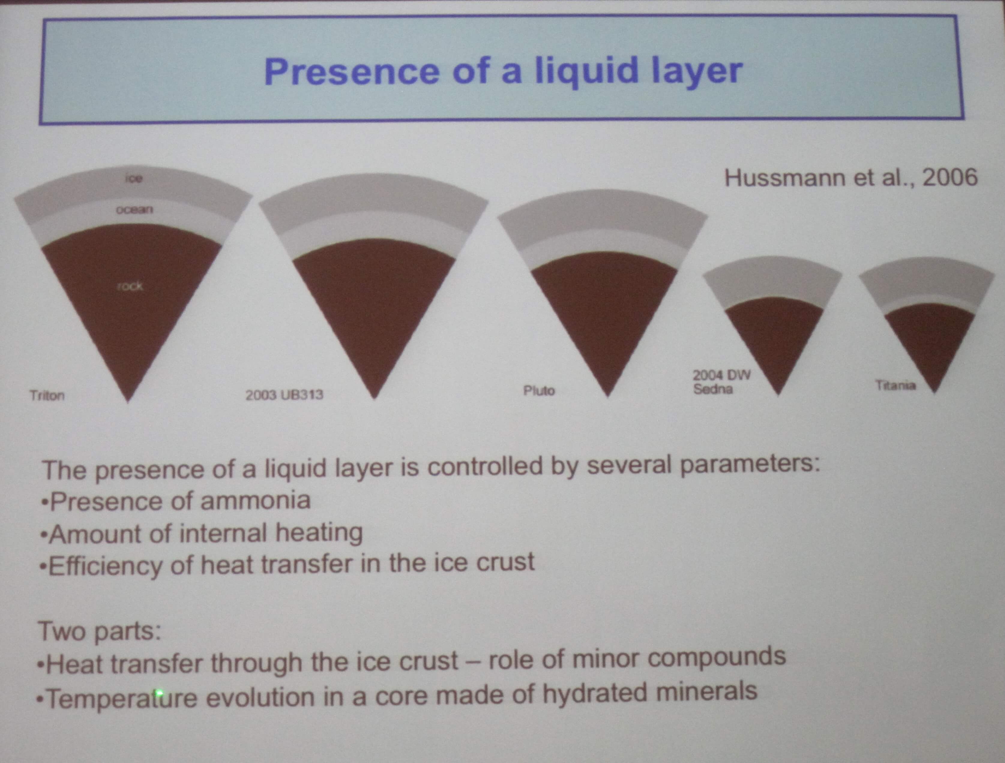
Geoffrey Collins (Wheaton College) “Predictions about Tectonics on Pluto and Charon.” His premise: “Tides raised by giant planets appear to be an important factor in icy satellite tectonics, but what about the Kuiper Belt?” He is interested in the time period after the initial Charon-forming impact. He and his colleagues have created models to calculate the interior viscosity for a range of Charon’s orbital evolution scenarios. They looked at the three main possible interior models for Pluto: (1) ice shell, ocean, rock core; (2) thick ice shell, rock core; and (3) uniform density. Another parameter they looked at was the formation distance of Charon from Pluto.

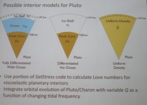
Possible interior models for Pluto are shown above: (left) ice-shell, ocean, core, (middle) thick ice-shell, core, (right) uniform density (undifferentiated).

Conclusions. Pluto will need to have an interior > 200 K. It  is likely that due to tidal heating (when orbital and rotational energy are dissipated as heat in the crust, which would be happening for Pluto despinning after formation), Pluto would melt and differentiate. The most self-consistent models include an ocean.

Beau Bierhaus (SwRI) talked about “Crater and Ejecta Populations on Pluto and its Entourage.” Craters are the most abundant landform in the solar system. They tell us about the target on/in which they reside. By studying the numbers and sizes of craters, and assuming an estimated impact rate, one can use crater density to estimate surface age. They are also indirect indicators of the impactor and in the case of Pluto, this could tell us information about the Kuiper Belt makeup.

Mass ejected from a crater follows an inverse relationship with velocity. Less mass is ejected at higher velocities, but to have ejecta (the material thrown out after an impact), the speed has to be above a particular Vmin, minimum velocity.  And if that velocity is lower than the escape velocity for an object (the speed above which would allow the object to escape the gravity well and go into orbit), you can create secondary craters. For ice, Vmin ~150-250 m/s. Pluto has Vescape ~1180 m/s; Charon has Vescape ~550 m/s. So we expect to see secondary craters on Pluto & Charon. Sesquinary craters might form when Vmin>> Vescape and the ejecta does escape the surface and then falls back onto its surface or onto another body. These are expected to be rare, but it’s possible you can have a crater formed on Pluto from a secondary ejected from Charon.

Predictions for New Horizons. Expect to see secondary craters on Pluto & Charon. Most of the craters will be primary impacts and they may have unusual morphology due to low impact speeds.

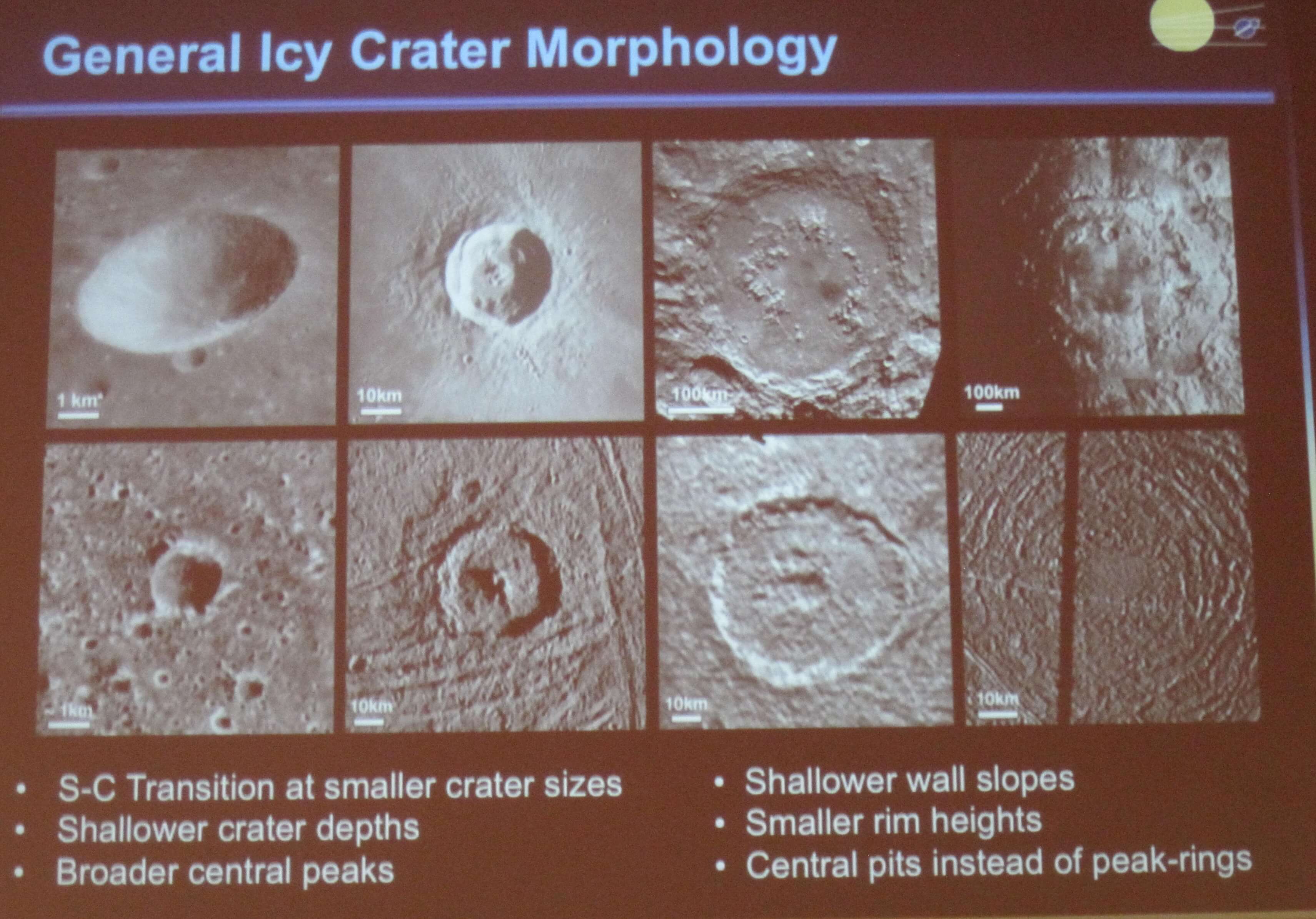
Veronica Bray (LPL, Arizona) continued the conversation with her talk on  “Impact Crater Morphology on Pluto.” The crater morphology (shape) depends on properties of impactor and also the gravity and surface/subsurface of the receiving body. For Pluto, we expect the crater morphologies to match those expected for impacts to icy bodies: shallow wall slopes, smaller rim heights, and central pit instead of peak-rings.

Comparative crater morphology. Top row: Impact Craters on a rocky body (Earth’s Moon). Bottom Row: Impact craters on icy bodies. Left to right indicate increasing crater diameter. The multi-ring basin, shown at the bottom right, is the Tyre crater on Europa, hypothesized to be the remnant of an object that penetrated into the subsurface.

Lower impact velocity will provide less impact melt. New Horizons will resolve large and small-scale features. However, with respect to things like Isis-style floor pits, New Horizon’s best resolution is not high enough.

What will New Horizons data tell us? New Horizons will address answers to how velocity affects peak development and primary crater depth, central pit formation in relation to melt drainage, and the d/D (depth to Diameter) trend to address heat flow models over time.

Olivier Barnoiun (JHU/APL) talk was entitled  “Surfaces Processes on the Moons of Pluto: Investigating the Effects of Gravity.” He is interested in processes on the smaller Pluto moons: Nix, Hydra, Kerberos, and Styx. He identified analogies in the solar system like 25413 Itokawa, a 100m asteroid that had been imaged by JAXA’s Hayabusa spacecraft in 2005. Hayabusa’s images revealed boulders that clustered together and were aligned; the leading hypothesis is that they were placed there by motion due to gravity. Other processes due to the presence of gravity, such as slope motions, are seen in the images. He notes that New Horizons will not have the resolution to duplicate the resolution Hayabusa had on Itokawa.

He and his colleagues have developed a computation “plate model” approach to tackle the motion of surface objects caused by “acceleration due to gravity” and this can be applicable to non-spherical bodies, for which Pluto’s smaller moons are highly suspected to be.

Marc Neveu (Arizona State University) asked “Exotic Sodas: Can Gas Exsolution Drive Explosive Cryovolcanism on Pluto and Charon?” Charon’s surface looks geologically young and could have an environment suitable for cryovolcanism. The term cryovolcanism was coined to explain the condition where the volcano erupts volatiles such as water, ammonia or methane, instead of molten rock . He presented a geochemical model where he has gas exiting a liquid as the mechanism for the cryovolcanism. The model involves the host liquid with different gas materials added and requires a crack in the surface ice layer. They also applied their model for a object that has a top crust; the crust acts like a “pressure seal” and prevents the gas from exsolving (separating from the liquid).

Lynnae Quick (JHU) presented some additional unique physics at Pluto with her talk on “Predictions for Cryovolcanic Flows on the Surface of Pluto.” She started with the statement that candidate bodies where cryovolcanism may be taking place are Enceladus, Europa, Titan and Triton. Imaging data from Voyager 2’s flyby of Neptune’s moon Triton provides strong evidence of cryovolcanism through interpretations of the terrain characterized by a lack of craters, geyser-like plume, walled plains, ring paterae (smooth circular), pit paterae, guttae (drop features).  She and her colleagues are modeling the cooling of (surface) lava flows and used a variety of “candidate lava compositions,” mixtures of H2O, NH3, CH3OH, CO, CH4, N2 ices. They compute cooling time for variety of lava thicknesses and compositions.

Predictions for Plutonian Lavas. Their work suggests N2-CO and/or N2-CH4 lavas could have 62-68 K melting temperatures, so essentially they could stay “molten” on Pluto for long duration. They will need high-resolution topography of Pluto, Triton, and Io, lab data for 50-273 K and New Horizons imagery of Pluto data to advance their models.

Alan Howard (University of Virginia) spoke about “Landforms and Surface Processes on Pluto and Charon. ” He walked us through multiple ways to add and subtract material from a surface:Accrescenence is the addition (e.g., condensation) of material normal to the surfaces, resulting in outward facing surfaces getting rounded and inward faces surfaces being sharpened.Decrescence is the removal (e.g., sublimation) of material normal from the surface, resulting in the outward facing surfaces being sharpened, and inward faces getting smoothed. Mass wastingis the bulk movement of material downslope aided by gravity (e.g. avalanches, debris flow, landslides). Gas Geysers are caused when solar energy hits ice, heating the underlying surface that then expands and erupts through the surface. Aeolian (wind) processes form things like sand dunes. To address this complex series of multiple surface activities, landscape evolution modelshave been developed to model such these processes with time.

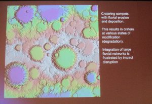
Result of a landscape evolution mode. Shown here is one result where large fluvial (flow) networks tend to get disrupted when you have a lot of impacting events.

Predictions for New Horizons. Expect to see scarps (steep banks) on the surface of Pluto. Expect to see the unexpected on Pluto and Charon.

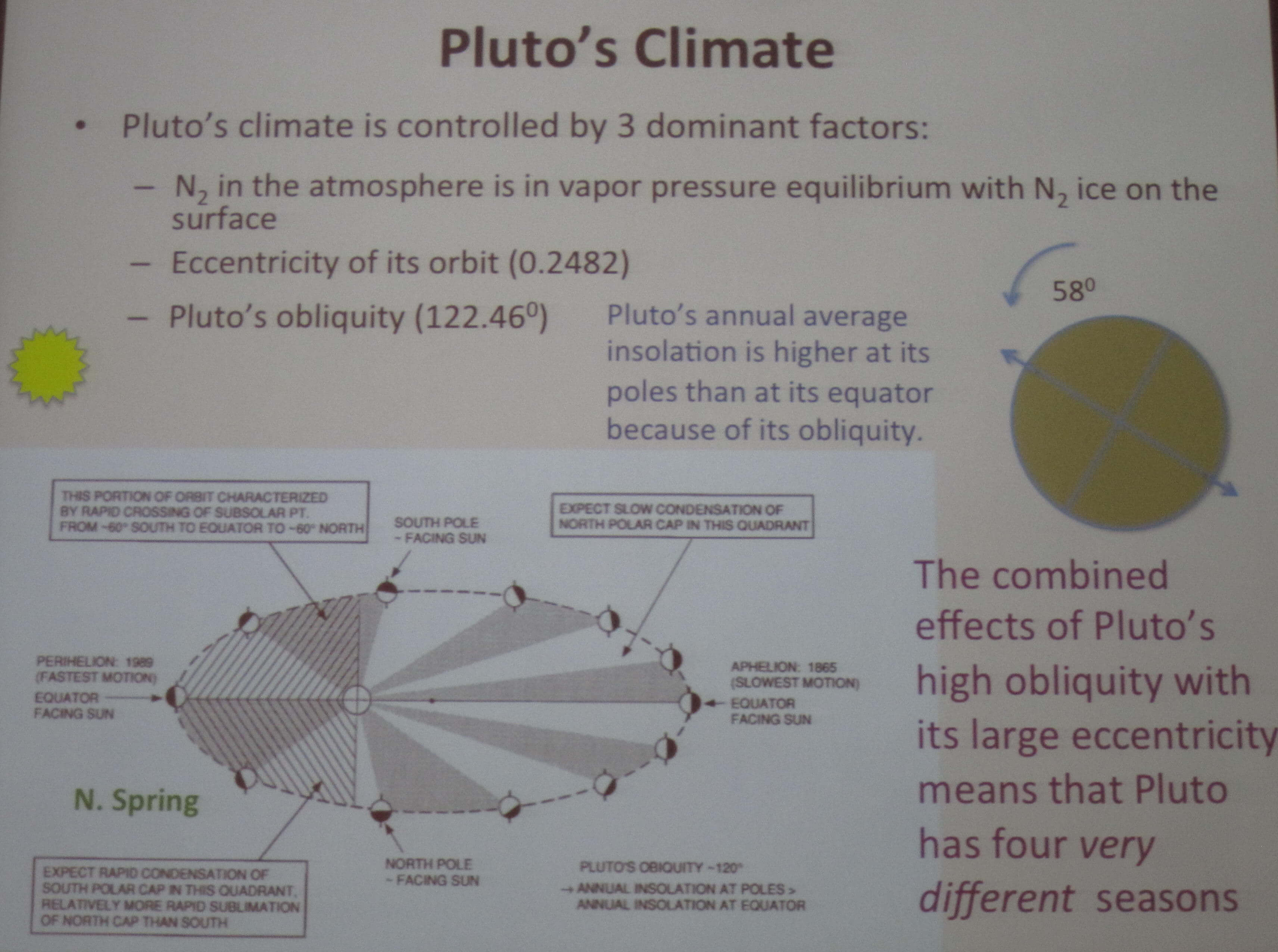
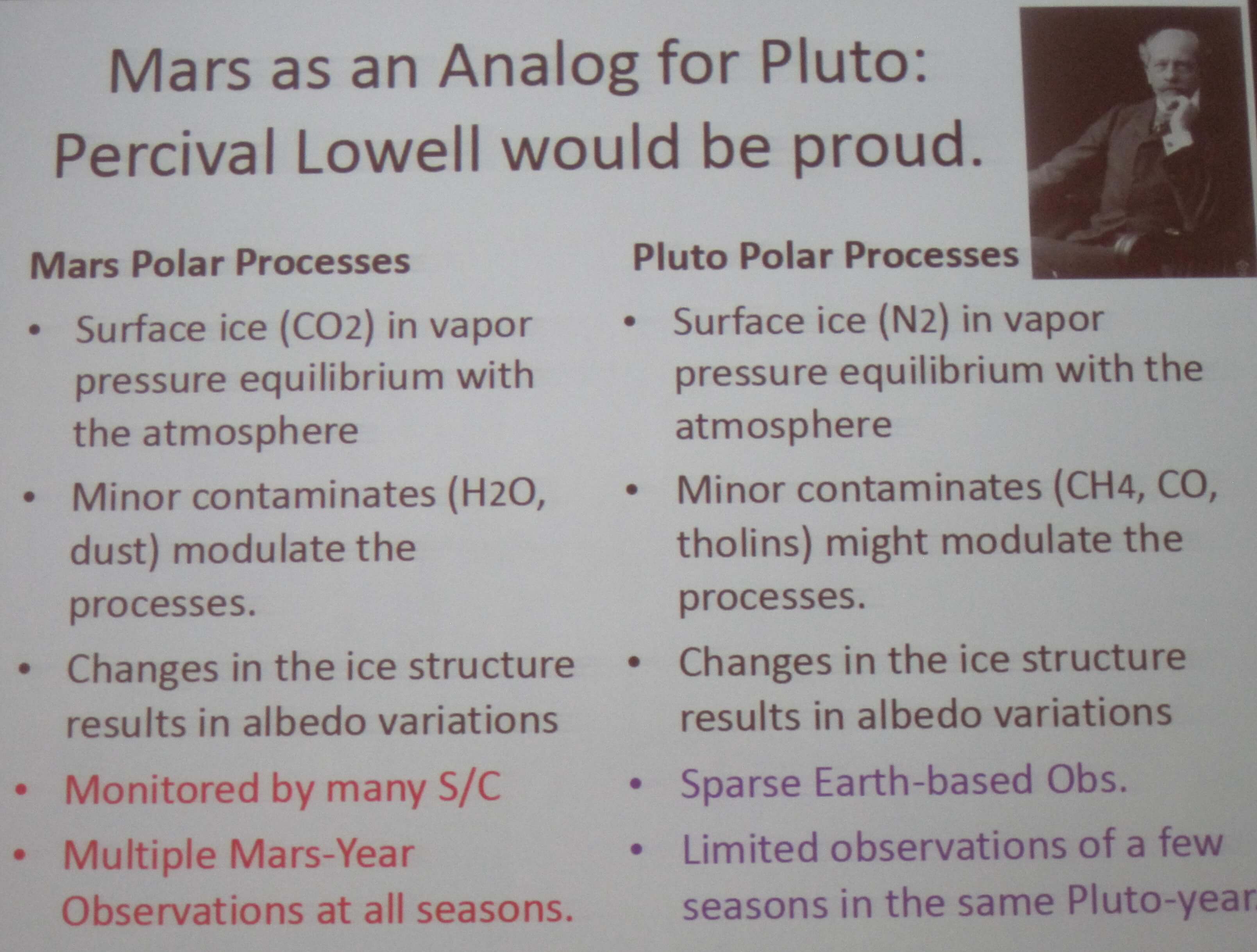
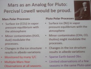
Timothy Titus (USGS) gave a thought-provoking talk about using the “Mars Seasonal Caps as an Analog for Pluto: Jets, Fans, and Cold Trapping.”  His premise is that the Mars’ polar processes are suitable analogs to explain what may be happening on Pluto. He stepped us through the Mars polar volatile transport model.

A key item is thermal inertia. On Mars the soil absorbs heat in summer, but high enough thermal inertia (200 MKS) to delay ice formation until late in the year, and this, as you would expect, affect the whole ‘ice cycle.’ There is a big disconnect in the community over what Pluto’s thermal inertia is. In E. Lellouch’s talk on Jul 23 (see earlier blog entry) he reported that Spitzer & Herschel have measured Pluto’s thermal inertia as 20-30 MKS (Lellouch et al 2011). However, Pluto atmosphere pressure models needed to match occultation by C. Olkin & L. Young require Pluto have a much higher thermal inertia >1000 MKS to explain their occultation measurements (presented at this meeting).

Thermal inertia is a measure of the ability of a material to conduct and store heat. In the context of planetary science, it is a measure of the subsurface’s ability to store heat during the day and reradiate it during the night. This has natural consequences for deriving what happens to processes that require an exchange of heat such as transport models. Thermal inertia measurements can also be used to infer types of surfaces, e.g. distinguish between fine dust/few rocks and coarse sand/many rocks. MKS is a short form for the units “J K-1 m-2 s-1/2.”

He makes a tantalizing comparison between the north/south asymmetry in the Mars polar ice caps due to topography and suggests whether this could possibly be an analog to why the methane and N2 have longitudinal distributions (shown yesterday in Will Grundy’s talk). Jets, plumes, fans, and spiders on Mars are results of active gas geyser activities. He postulates, could the same be occurring on Pluto? If we miss the gas/plume season, we could see the leftover signatures in fans and spiders.

Predictions for New Horizons. Asymmetric seasonal caps. Methane lags surrounding the Nseasonal cap. Optically thick layers of methane on top of N2 ice. Solid green house gas jets or at least spiders and fans.

David Williams (Arizona State University) talked about “Using Geologic Mapping as a Tool to Investigate the Geologic Histories of Pluto and its Satellites.” Geologic mapping documents the main geologic units and features and their relative ages and other characteristics. This is an iterative process using greyscale images, topographic data, and compositional and spectral data. They also identify structural features (crater rims, ridges, toughs, graben, lineaments, scarps, pits, etc.) They can use crater model ages to define a model-derived stratigraphy. The Geologic Information Software (GIS) is used to make the maps. Geologic maps are being made of the Moon, Jupiter system, Saturn system, Mercury, etc. from orbiter data. Data from fly-by missions have been used to make maps, such as Mariner 10 (Mercury), Voyager-Galileo (Galilean satellites), Cassini RADR (Titan). There will be a challenge of the vastly changing resolution data sets from the New Horizons flyby, but they would like to make these maps.

John Spencer (SwRI) ended the session with “What will Pluto Look Like?”  He began, “Will Pluto Look like Triton?” And his answer: Geologically, Yes.  He does not expect to see lots of craters. He expects that Pluto will have a surface that is as young and geologically active as Triton’s. One of the surprising thing about Triton’s surface is that it is lightly cratered. Are we seeing a situation where Triton had been completely resurfaced a lot since its capture by Neptune? And it should also have sufficient internal heating from radiogenic heating (radioactive decay from rock) rather than rely on Neptune to provide resurfacing mechanisms.

When looking at albedo (reflectance) contrasts between Triton (Voyager 1989) vs. Pluto (HST data 2004), you see factors of 10 across short distances on both bodies. Non-volatile surfaces on Triton are “bright” explained as H2O and CO2 exposed.  However non-volatile surfaces on Pluto are “dark” explained as H20 and CO2 buried by dark material. So Pluto will not look compositionally like Triton. John Spencer then drew our attention to Iapetus, a moon of Saturn, that also has a range of albedos, dark to light, with the hypothesis being an “exogenic trigger” and was suggestive of an analog there.

In answering a question about a prediction for topography, the discussion led to Paul Schenk (who spoke earlier) suggesting that Charon would look pretty flat (like Triton), with +/- 1km range. Bill McKinnon reminded us that Iapetus is an example of a body with extreme topography, ~ +/- 15km.

After such a visualizing intriguing morning, one thing can be certain: Pluto and Charon surfaces will have an impact (pun intended!) on our understanding the nature of icy bodies in our solar system.

It’s more than skin deep. Interiors of Pluto and Charon, a Discussion.

Reposted from https://blogs.nasa.gov/mission-ames/2013/07/26/its-more-than-skin-deep-interiors-of-pluto-and-charon-a-discussion/.

This entry is a summary of talks presented at the Interiors session July 24th, 2013, during the Pluto Science Conference in Laurel, MD being held this week July 22-26, 2013.

Christophe Sotin (JPL) began the session with a talk entitled “Processes involved in the evolution of Pluto’s interior Structure.” He started his talk with a comparison of model of the interiors of Ceres, Callisto, Enceladus, Pluto (McCord & Sotin, 2005; McKinnon & Mueller, 1986; and Simonelli & Reynolds 1989). More recent models propose the existence of a liquid layer between an icy surface and a rocky core (Hussman et al 2006). This layer of liquid changes the way heat is transferred to the ice crust. If liquid methane could form at the base of the ice layer, forming a “sub surface ocean”, it would react with water and form stable methane clathrates. The presence and thickness of the “clathrate layer” affects the thickness of the ice crust above it.

Conclusions. In their interior models, minor components (e.g. NH3) play important roles in both the characteristics (e.g. thickness) and dynamics of the ice crust. They need laboratory experiments to study the relative stability of the clathrate hydrates.  Hydrated silicates (e.g. antigorite) are likely to be the make-up of the Pluto core.  It will undergo dehydration some 100 Myrs to Gyrs after accretion. Convection within the core. The presence of a subsurface ocean depends on the presence of minor components.

The term clathrate is used to describe a structure that consisting of a lattice that traps or contains molecules.

Francis Nimmo (UC Santa Cruz) followed to provide some suggestions of surface observational evidence to probe the “Interiors of Pluto and Charon.”

Shape is Important. Shape tells us whether a body responds like a fluid. If the body behaves like a fluid (i.e., behaves hydrostatically), you can compute the moment of inertia. This, in turn can tells us something about the interior (i.e., is it differentiated or not). There is a caveat that differentiation can also occur due to radioactive decay. Differentiation happens when ice melts, so it tells us about thermal evolution.

Comparative study of other bodies in the outer solar system and what we know about their interiors.

Evolution of Shapes. Early on, Pluto & Charon are rotating quickly, and are distorted. Pluto and Charon change shapes in the first few to 100 Myr if fluid or elastic, respectively, as their spin rate slows down and Charon moves outward. The spin rates influence their shapes.

What leads to Oceans? A conductive (no convection) ice shell is required to make an ocean (Desch et al 2009). This shell basically lets the heat out from the core. This heating then melts the bottom of the ice shell creating an ocean. The presence of an ocean changes the stress history. In the creation of an ocean, you are replacing low-density ice with higher density water and this introduces compression stresses. If you see things like the Tyre crater on Jupiter’s moon Europa, a multi-ring impact that implies there was an ocean. Whether or not an ocean is present has important astrobiology & geophysics consequences. If you introduce an ocean, you never have a fossil bulge. If you do not have an ocean, you could get a fossil bulge.

A fossil bulge is a bulge that froze into shape before the satellite synchronized its rotation.

Martin Paetzold (Universitat zu Koln, Germany) spoke about “Mass Determination of Pluto and Charon from NH’s REX Radio Science Observation.” During the fly-by, Pluto will perturb the New Horizons spacecraft velocity just slightly and this will be recorded as a tiny Doppler shift of the X-band (8.4 GHz) radio carrier frequency. This information will be used to measure the mass, or more specifically, the product GM (universal gravity constant times the mass), of Pluto.  There are two different ways to obtain this data during the New Horizons mission: (1) Using two-way ranging a week before the encounter and week after the encounter, and (2) During the encounter, the REX uplink instrument (operating at 7.1 GHz) will have a series of measurements during the days around closest approach. They hope to obtain 0.15% accuracy for the first method and 0.04% for the second method. The best results utilize both methods potentially deriving an estimate of Pluto & Charon masses with an accuracy of 0.01%. They are currently looking at the small forces file, which is the measure of the attitude performance during thruster firing.

James Roberts (JHU/APL) spoke about “Tidal Constraints on the Interiors of Pluto and Charon.” Thermal evolution of Pluto & Charon is a key question for scientists to answer. But thermal models are dependent on interior structure. At present we do not know whether Pluto or Charon are homogeneous (i.e. same material throughout) or differentiated (split into a core and crust, or maybe core, subsurface ocean and crust). Typical methods used to probe interiors are Kepler’s 3rd Law, Bulk density, Moment of Inertia, Gravity, Magnetism, Radar, Seismology, Tides. For New Horizons, as the fly-by is not that close, Gravity is not a viable method; the lack of a magnetometer aboard rules out Magnetism, and Seismology requires the spacecraft to land, also not possible. He described their approach  that will use Shape Modeling to measure a Tidal Bulge. Both Pluto and Charon may each raise a tidal bulge on the other. He cautioned that we may not be able to determined the existence of an ocean using a shape model.

Steve Desch (Arizona State University) spoke on “Using Charon’s Density to Constrain Models of the Formation of the Pluto System.” The unique Pluto-Charon system has been modeled as arising from the impact of two large Kuiper Belt Objects (KBOs). This had been presented on July 23rd by Robin Canup. Steve Desch’s model takes two differentiated KBO bodies (but they must have a thick crust) in a disk and collides them. Parts from the bodies’ inner core, plus some ice, forms Pluto and the outer icy mantles form Charon & the other moons. He addressed that the initial differentiated KBOs with r=600-1200 km could exist (Desch et al 2009, Rubin et al 2013). The outcomes of this model create a dense Charon (density= 1.63 g/cm3) because Charon would have been formed from the outer regions of the initial KBOs, and those objects are characterized with thick crusts.  This is the alternative model that was not preferred by Robin Canup in her talk yesterday. This remains an active area of study.

Wrapping up this 3rd day of a dynamic conference we learned that we still have a lot more questions about the formation and the interior or Pluto, Charon or any of these icy bodies in the Outer Solar System. New Horizons will indeed bring an revolutionary dataset to allow to direct investigation of surface features, overall shapes, masses, and orbital dynamics, all which will constrain models of what these bodies are made of and how they formed.

Some insights into Charon and what roles laboratory work can play in New Horizons science.

Reposted from https://blogs.nasa.gov/mission-ames/2013/07/26/some-insights-into-charon-and-what-roles-laboratory-work-play-in-new-horizons-science/.

These are talk summaries from the afternoon of July 24th at the Pluto Science Conference being held this week, July 22-26, 2013 at the Johns Hopkins University Applied Physics Lab in Laurel, MD.

Marc Buie (SwRI) walked us through “The Surface of Charon.” Charon was detected by Jim Christy in April 1978, in what were originally dubbed “bad images” from the Naval Observatory, but not confirmed as a satellite by the IAU until February 1985. Charon is about 1 arcsecond from and ~1.5x mag fainter than Pluto. An occultation measurement in April 1980 confirmed the detection.

“Mutual Event Season” is when every half orbit of Charon passes in front or behind Pluto. This occurred over 1985-1990 time frame. For the specific orientation where “Charon went behind Pluto,” as observed from Earth, you can directly measure’s Charon’s albedo, the size ratio between Pluto and Charon and start deriving its composition. So, work in earnest to determine Charon’s surface started in the mid-1980s.

In 1987, Marc Buie and his colleagues got IR spectra using a single-channel detector and a circular variable filter, the best in spectrographs at the time, and this revealed Pluto’s atmosphere is methane dominated and Charon’s atmosphere is water dominated, and they do not look like each other.

Hubble Space Telescope (HST) entered the scene and a series of observations of Pluto and Charon with HST started in 1992. The first rotational light curve of Charon was obtained in 1992-1993, indicating a 8% variation in the brightness, much smaller than that for Pluto and the data also confirmed that Charon was tidally locked with Pluto (just like our Moon is tidally locked with Earth, showing the same face). Marc Buie and his colleagues obtained HST NICMOS near-infrared spectrum in 1998 of both Pluto & Charon.

Comparison of Pluto and Charon infrared spectra, taken in 1998 at the same epoch (near in time with each other), with HST NICMOS (near infrared camera and spectrometer aboard Hubble).

A mystery. Spectra from Tethys, one of Saturn’s moons, has a remarkable agreement with Charon’s spectra, despite the bodies are of different temperatures and albedos? Will they have similar compositions when the New Horizons spacecraft flies by? The spectra is also not fit precisely with just water, so there is another unidentified species there.

Marc Buie was observing Pluto & Charon just last night (July23rd, 2013) with the Adaptive Optics mode of the OSIRIS instrument on Keck. This instrument achieves comparable spatial resolution as Hubble. At the conference, he showed off the latest image, “hot off the press.”

Predictions for New Horizons: Charon to have a heavily cratered surface with modest (subtle) albedo and color features. Expect to see differences between the Pluto and anti-Pluto hemispheres.

Francesca DeMeo (MIT) talk was entitled “Near-Infrared Spectroscopic Measurements of Charon with the VLT.” She began her talk stating that TNOs (Trans-Neptunian Objects) can be characterized  as (1) volatile-rich (lots of N2, CO, CH4), (2) volatile-transition, (3) water+ammonia rich (H2O, NH3), and (4) volatile-poor (neutral to very red colors, maybe some water ice). No TNOs, to date, show evidence for CO2. Her analog is to Charon is Orcus, a TNO with its own moon Vanth. Both are water and ammonia-rich bodies.

Comparison of two water and ammonia-rich bodies: the TNO Orcus and Pluto’s moon Charon.

She observed  Charon in 2005 using the VLT (8m telescope) with AO (adaptive optics), which separates Pluto. Her Pluto data is published in DeMeo et al 2010. Charon data was presented here in her talk and showed a comparison with Jason Cook’s data from 2007 and F. Merlin’s data from 2010, as they were looking at the same surface location. She is using the JPL Horizons longitude system.

For a review of Trans Neptunian Objects, she recommends Mike Brown’s 2012 Review Paper http://adsabs.harvard.edu/abs/2012AREPS..40..467B.

Gal Sarid (Harvard) followed with “Masking Surface Water Ice Features on Small Distant Bodies.” Minor (icy) bodies (TNOS, Centaurs, comets) are a diverse population with varied size, composition and structure. Their surface compositions show evidence for water ice and other volatile species. They are understood to be remnants of a larger population of planetesimals. He stepped us though his thermal and physical model of a radius=1200km object to reveal the possible insides of these minor icy bodies. Observationally this could be tested by inspecting impact crater that could eject subsurface material. From his computations he varies the ratio of carbon (dust) to water ice to give predictions for water band depth. When he compares the colors of the computed spectra they match very ice-rich TNO bodies, but his work reveals questions to explain the B-R colors. The models may need more other ices (methane, methanol).

Reggie Hudson (NASA GSFC), a laboratory spectroscopist, presented  “Three New Studies of the Spectra and Chemistry of Pluto Ices.” At NASA Goddard, they have equipment to test ices with their vacuum-UV (vacuum-ultraviolet).  He showed 120-200 nm results of N2 + CH4 at 10 K. A second study was to measure CH4 ice in the infrared. CH4 has three phases: high temp crystalline T > 20.4 K, low temp crystalline T < 20.4 K, and amorphous CH4 forms around 10 K. He showed results for solid CH4 from 14-30 K over 2.17 to 2.56 microns and 7.58 to 7.81 microns. Their lab also has the ability to irradiate the samples, and when they have done so, certain phases recrystallize, but that is a function of temperature. Future work involves completing lab data of C2H2, CH4 and C2H6. Their lab website is http://science.gsfc.nasa.gov/691/cosmicice/.

Brant Jones (University of Hawaii) discussed  “Formation of High Mass Hydrocarbons of Kuiper Belt Objects.”  They irradiate their ices with a laser and their measurement technique is a “Reflectron time-of-flight mass spectrometer.” They have identified 56 different hydrocarbons wit their highest mass C22Hm where 36 < m < 46. Future work is to investigate PAHs, look at “processed ices” and study different compositions, and study exact structures.

Christopher Materese (NASA Ames) spoke on “Radiation Chemistry on Pluto: A Laboratory Approach.” Reporting on their laboratory work at NASA Ames, in their setup, they radiate their ices with ultraviolet (UV). Now for Pluto, the atmosphere will be opaque (not-transparent) to UV radiation. Secondary electrons generated by ion processes, however, drive the chemistry and their energy (keV-MeV) is similar to that provided by UV radiation. He presented NIR (near infrared) and MIR (mid-infrared) spectra of his irradiated ices. They have completed over 20 molecular components. They also have a GC-MS (gas chromatograph–mass spectrometer) to measure the masses of the molecules they create.

The importance of laboratory work cannot be underestimated. It can help with predictions and equally important help with identification of molecules. Then once molecules and their abundances are determined, that can fold into more complicated models to look at volatile transport.