Reposted from https://blogs.nasa.gov/mission-ames/2013/07/24/how-can-you-form-pluto-and-charon-let-me-just-count-the-ways/.

On the afternoon July 23, 2013 at the Pluto Science Conference continued, we switched gears from atmospheres to small satellites. This blog entry is about the formation theories for Pluto and Charon.

Hal Levison (SwRI) started the afternoon with a talk entitled “Unraveling the Early Dynamical Evolution of the Outer Solar system.” The “Nice Model” (Gomes, Levison, Morbidelli, Tsiganis) was devised to introduce possible models that could produce the Outer Solar System as we know it and preserve the Inner Solar System as we know it. The authors have been updating it with planets in resonances (Morbidelli et al 2007), put Pluto-objects in the disk (Levinson et al 2011), restricted the models to “save the Earth” by making sure Jupiter does not encounter an ice giant planet (Brasser et al 2009), and added a third ice giant (Nesvorny & Morbidelli 2011).

To learn more information about the Nice Model, check out a good entry at http://en.wikipedia.org/wiki/Nice_model.

The Nice model has told us a lot of good things. It predicts the right number and range or orbits for Jupiter and Saturn, predicts the right number and orbits for Trojans (things in 1:1 resonance with primary body) and reproduces the Late Heavy bombardment of Moon. However, it comes short of explaining the Kuiper Belt.

So, what does this all mean for the Kuiper Belt? The Kuiper Belt is a rich structure. Observationally the sum of all the mass in the Kuiper Belt is <= 0.1 Mass_Earth.  In order to get objects the size of Pluto to grow in the timescales of our Solar System, you need a lot more mass. So we need find this missing mass.

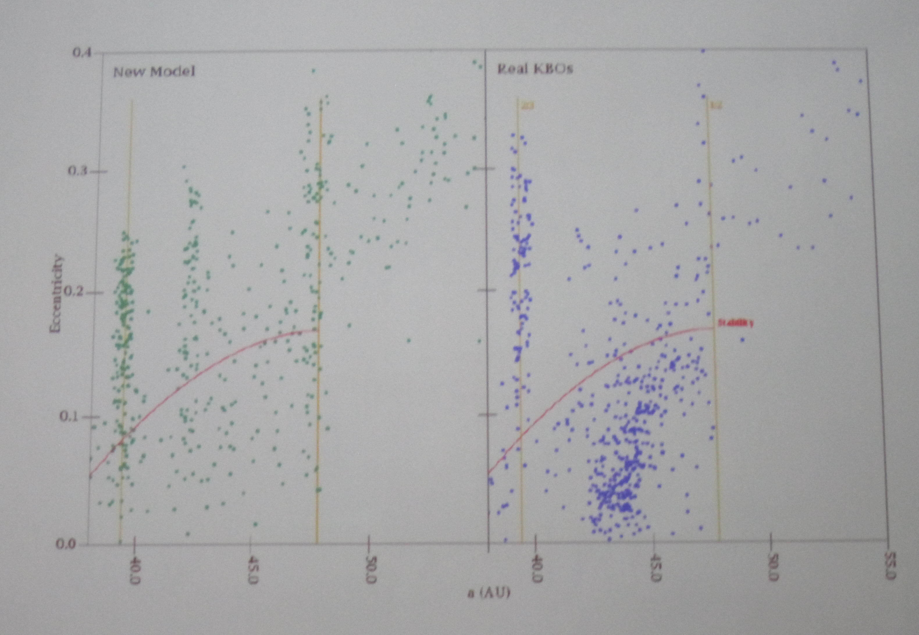
Above is a Comparison of updated 2008 Nice Model (green ) vs. Kuiper Belt Data (blue dots). It qualitatively shows similarities however it cannot reproduce the “kernel” (described in Brett Gladman’s talk from July 22nd) nor objects with high inclination (large i) nor objects in the “Cold Classical Population.”

Cold Classical Kuiper Belt Objects have orbits much like the planets; nearly circular, with an orbital eccentricity of less than 0.1, and with relatively low inclinations up to about 10° (they lie close to the plane of the Solar System rather than at an angle). They have characteristics similar to an undisturbed protoplanetary disk. Often the term ‘primordial’ is used when describing Cold Classicals. They tend to be in binaries and have “red” colors.

He then ended his talk by sharing an recent update with his work on Outer Solar System modeling, hoping to explain high inclination Kuiper Belt Object formation, by looking at the formation of Jupiter and Saturn with and without a gas disk present. Jupiter and Saturn, when they are forming, are scattering objects outward. Then if there is a gas disk present, these objects get into what is known as Kozai resonances, where bodies exchange eccentricity for inclination. As the gas disperses, a population at high inclinations in the Kuiper Belt region (30-50 AU) are caught. In the models, if you vary the outside extent of the disk, you spread out the populations. However, this is not in agreement with our solar system (we don’t see those types of objects). Their conclusion is that you needed to have the gas disk truncated and this modification of the Nice Model can explain high inclination KBOs.

Hal Levinson stated strongly “We definitely need New Horizons to visit a cold classical object!”

Anders Johansen (Lund University, Sweden) in “Accretion of Kuiper Belt Objects” stepped us through the two models of major planet formation: Planetesimal (coagulation) vs. Pebble (steaming instability).

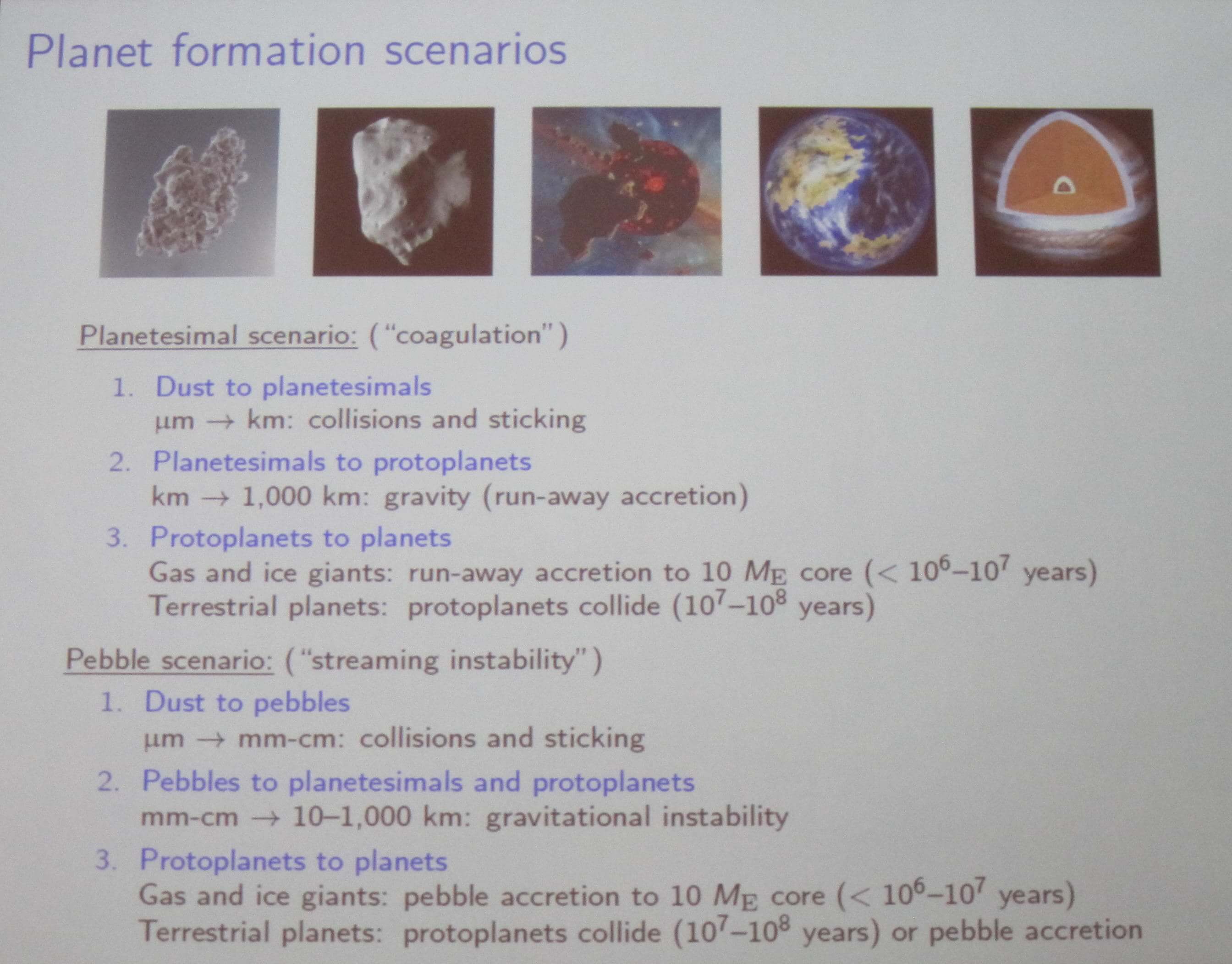
He asked, could Pluto be formed by planetesimal accretion? This will require a cold disk of km-size planetesimals (Kenyon & Bromley 2012) where a key prediction of the planetesimal accretion model gives a differential size distribution that is in agreement with observations (i.e. lots of smaller objects). But, there is a problem this this approach since to make kilometer size objects beyond 20 AU as it would taken 100 Myr which is much longer than the life-time of the gas disk (Lambrechts & Johnansen, in prep). Thus, to make a Pluto-size (few 1000s km size) object would taker longer than the age of the Solar System. (Pluto orbit is 29 AU at closest to Sun to 49 AU, furthest from Sun). However adding streaming instability can speed up the planetesimal growth timeframe.

Could Pluto have been formed by pebble accretion? Pebbles are accreted very efficiently by planetesimals (Lambrechts & Johnansen,  2012; Ormel & Jlahr 2010). This shapes the distribution (makes it steeper) and brings it more into agreement with asteroid and KBO populations.

What new data will New Horizons shed? If data from New Horizons reveals the presence of Aluminum 26, this will imply a formation age for Pluto. Formation time data can be fed back into planet-forming models, be they planetesimal or pebble accretion, and those models can be used to help explain other systems, such as observed proto-planetary disks or exoplanet systems around other stars.

Robin Canup (SwRI) talked about the “Origin of Pluto’s Satellites.” Massive Charon and four very tiny outer moons make up Pluto’s satellites. All of these satellites are co-planar (they are moving in the same plane) and prograde with respect to Pluto’s rotation (they revolve about Pluto in the same direction as Pluto’s rotation). However, Pluto’s rotation is retrograde (in the motion opposite) to its orbit.

It is thought that Charon was formed by a giant impact that could have preserved a lot of angular momentum in the system. Her models (Canup 2011) predict a grazing impact was needed to match the system angular momentum and produce a Charon-mass object. Achieving a Charon-mass object requires an extreme case, as most of them like to create a companion that is 6-8% of mass of the primary object.

She also modeled cases where there is an undifferentiated impactor, and those systems can form “intact-moons.” In many scenarios, Charon-mass objects are created. And “the Charon that was created” forms entirely from impactor material. She postulates that this is the more probable explanation for Charon’s formation.

What about the origin of the tiny moons? The models do create a disk, which has enough mass to form tiny moons. The challenge is that the disk that is made too compact compared to the current existence of Nix & Hydra. Could these moons have been transported out? But no model has been able to drive them out via “resonant transport.”

The alternative theory for the formation of the smaller moons is by capture, but it’s rather very low probability. Plus that could imply far more irregular satellites and Pluto’s smaller moons are more regular. So this opens up the path for other theories. Collisional spreading? Collisional dampening? Preferential re-accretion?

This is an active area of study.

How New Horizons can help. By providing better constraints on masses and densities of Pluto & Charon, compositions of the tiny moons, any information about the differentiation shape of Pluto & Charon, and presence of distance satellites can better constrain these origin model.

Reposted from https://blogs.nasa.gov/mission-ames/2013/07/24/more-predictions-about-plutos-changing-atmosphere-and-charon-may-have-a-few-surprises-of-her-own/.

Blog series continues. These are summaries of talks presented on July 23, 2013 at the Pluto Science Conference. The New Horizons mission will fly by the Pluto System on July 14, 2015, a place that has never been explored before by any other spacecraft. Many questions about the Pluto System remain unanswered. For more information about NASA’s intrepid explorer to the Solar Systems’ Third Zone go to http://pluto.jhuapl.edu/ and http://www.nasa.gov/mission_pages/newhorizons/main/index.html.

Richard French (Wellesley College) presented a talk on “A Comparison of Models of Tides in Pluto’s Atmosphere and Stellar Occultation Observations.”

We have come to understand that Pluto’s atmosphere is cold & tenuous, has a long radiative time constant, shows weak diurnal variations, indicates seasonal transport of volatiles with long term variations of atmospheric mass, and seems to be convectively stable. Current Pluto general circulation models (GCMs) predict smooth T(P) profiles reveal mean circulation and thermal structure. But there are problems. GCMs predictions (with these smooth T(P) profiles) are inconsistent with stellar occultation data, which imply much more complex T(P) profile. The other challenge to this mystery is that stellar occultations are spatially constrained (i.e., map across a particular lat/long swath of Pluto surface at the time of event).

Are there waves in Pluto’s atmosphere? This is one proposition to explain the structures (spikes) seen in the Pluto occultation data. Tidal models they have built make predictions for large scale and small-scale structures. Also they can predict temperature profiles with altitude. Next steps are to apply this model to other occultation geometries. Richard French showed a comparison of a tidal model (Toigo et al 2010) against occultation data from an event on Aug 21, 2002 and they showed qualitative agreement.

Richard French’s predictions for New Horizons fly-by: When New Horizons provides a true frost pattern, they can input this into their models and generate large-scale and small-scale structures for comparison with actual New Horizons atmosphere measurements. Their tidal models do generate regionally variable, latitude dependent thermal changes. If this is what New Horizons observers, their model can help constrain parameters.

Bruno Sicardy (Observatoire de Paris, France) next took us on a rich tour of “Pluto’s Atmospheric Pressure From Stellar Occultations: 2002-2012.”

There was a dual Pluto & Charon occultation event on 4 June 2011. Pluto and Charon each pass in front of the star (at different times). Look at curve shapes. Charon’s curve sharply drops, indicative of no atmosphere, unlike Pluto’s curve, which has not-as-steep ingress/egress that indicates the presence of an atmosphere.

Using the light curve data, Sicardy and his team use a temperature vs. altitude model to fit the light curve depth, width and ingress/egress slope. Then with the temperature, they can derive a pressure. He presented results from the most recent Pluto occultation that was observed May 4, 2013. Good data and good fit. Next were shown the derived pressure (at 1215km) for occultation events observed from 1988 to 2013.

Occultation results show the Pluto atmosphere is increasing over the past few years. There is some notable evolution and implies a regular expansion. But a question from the audience stressed caution as we could be seeing just the northern pole facing the Sun with that contributing to the expansion but it could be a localized phenomena.

Bruno Sicardy’s predictions for New Horizons fly-by: Atmosphere will be present for the fly-by.

Michael Person (MIT) next described “Trends in Pluto’s Atmosphere From Stellar Occultations.” He started his talk with the advantages of occultation measurements:  you get spatial resolution (~1 km at Pluto) with direct measurements of atmospheres (temperature, pressure, number profiles). MIT has collected data sets from 1988 through 2013. Their group tends to separate the upper vs. lower atmosphere when they fit their data. He next showed a light curve comparison over. Are we seeing a gradually decrease lower atmosphere slope? Is there a gradual lowering of the separation boundary?

“Haze or No Haze? That is the question.” Best evidence of haze is from the occultation event of 2002, where there is a distinct change in brightness as a function of wavelength (Elliot et al 2003).  Attempt to look for haze in the 2011 occultation event with SOFIA in three bands was not successful. The main question is why does the haze come and go, and what is causing it?

What Mike Person is looking forward to: New Horizons will finally provide the size of Pluto! Knowing where the Pluto surface really is, or equivalently, the size of Pluto, is a key data point, as all these interpretations of occultation light curves and interpretations to atmosphere assumes a Pluto size.

Alex Dias de Oliveira (Observatoire de Paris, France).“Pluto’s Atmosphere from Jul 18, 2012 stellar occultation.” This is his PhD work and he provided an updated status of the steps taken from prediction of the event, the observation data collected, various calibration items, and first attempts to invert the light curve to get a temperature profile. He observed this Pluto occultation event with the ESO VLT (8m telescope in Chile) with the NACO instrument in the H band (1.65 microns). Comparison with the June 12, 2006 AAT event showed that spikes seen in the light curves were repeated in the July 18, 2012 event he observed wit the VLT in Chile.

Cathy Olkin (SwRI) presented results from “The May 4^th, 2013 Stellar Occultation by Pluto and Implications for Pluto Atmosphere in 2015.” This was an event where Pluto passed in front of a R=14.4 mag star with a slow shadow velocity of 10.6 km/s. The event was observed from the southern hemisphere, from Cerro Tololo in Chile.

Erika Barth (SwRI). “Is Methane Supersaturation Consistent with the Presence of Haze Particles in Pluto’s Atmosphere?” She asked the question: If you put haze particles into Pluto’s atmosphere how do they interact with the methane in Pluto’s atmosphere?” She developed a model to ingest haze particles into a supersaturated environment and this predicts the growth of clouds and condensation of methane. Then when methane condenses out, that reduces the amount of observable methane. Her model requires the existence of a troposphere (which we learned earlier in Emmanuel Lellouch’s talk today that there is no evidence for this, but its existence could explain some phenomena, some observed to date, other predicted) and also predicts a thick troposphere as well. She created a Pluto version of CARMA, the Community Aerosol and Radiation Model for Atmospheres.

Jason Cook (SwRI) next spoke about his “Analysis of High Resolution Spectra of Pluto: A Search for Cold Gaseous Methane Layer, and Spatial Variation in Methane Column Abundance.” Occultations have told us that Pluto’s upper atmosphere (above 1195 km) is pretty warm (100 K). But 2.15 micron N₂ ice measurements of Pluto’s surface tells us the surface is ~40 K. So this implies there needs to be a cold-layer in the atmosphere. To investigate a search for this “cold layer of air” they took NIR (near infrared) spectra with NIRSPEC on Keck with R=35,000 in 2011. They need to move to a two-temperature model to help constrain the observed data (i.e. measured methane line depths from the high-res NIR spectra), but the hot/cold ratio of the two temperatures is an unresolved topic (pun intended).

They also took spectra of Pluto over several nights to probe the different longitudes of Pluto (Pluto has a rotational period of 6.4 days) and they got a fairly consistent number except near 180 deg longitude where gaseous CH₄ was not easily detected. They would like more data to probe this temporal measurement.

Selection of high-resolution NIR spectra of Pluto obtained over several days. This series probes a range of Pluto rotations and show how methane lines (Q-branch) vary.

Eliot Young (SwRI) spoke about “Evidence for Recent Change in Pluto’s Haze Abundance.” Hazes have been observed on Titan (photolysis products from higher up in the atmosphere) and Triton (condensates from surface). The August 21, 2002 occultation showed evidence for haze (change in brightness with color, Elliot et al 2003), but 2007 (0.51 & 0.76 micron) and June & July 2011 occultation events in different bands (I & K bands) showed no change in color.

Occultations can only probe down to a certain depth, so they are limited. We don’t really how close you got to the Pluto surface. If you have a special case where you can have a central flash or sets of flash spikes, you can derive more information. By applying a new technique on the 2007 Mt John light curves, he proposed they can determine amount of haze by evaluating the attenuation in those parts of the light curve.

Central Flash Description:  A central-flash occultation is visible when the observer is located near the center of the shadow path of the object. It is here where the atmosphere near the edges of the occulting body (for Pluto occultations, this is Pluto) refracts extra star light (from the background star) directly opposite from the star, forming a “brightening” in the middle of the deep light curve.

Mark Gurwell (Harvard CfA) provided a talk entitled “Atmosphere CO on Pluto: Limits from Millimeter-Wave Spectroscopy.” Carbon monoxide (CO) is expected based upon the presence as an ice on its surface. The first direct detection of CO was done in the NIR with the VLT (Lellouch et al 2011). Then JCMT (Greaves et al 2011) revealed a CO(2-1) line in the submillimeter, but this line had not been there a few years back, leaving a mystery. There is still mystery in fitting the CO abundance based on the measured submillimeter width and strength of this line. He did show that Pluto had been in the fore-ground of a galactic emission during the JCMT observations. He supposes that they had contamination. They did their own observations using the SMA sub-millimeter telescope multiple times and did not detect the CO(2-1) line in the spectra (they have upper limits). So he is excited about using the ALMA array that has 30-50x SMA sensitivity to really address the CO, nitriles and isotopes.

And the final talk of the morning Atmosphere session just could not leave Charon out of it.

Alan Stern (SwRI) “Cometary Impact Produce Transient Atmospheres on Charon.” Most scientists have come to accept that Charon does not have an atmosphere (see earlier posting in Bruno Sicardy’s talk showing the dual occultation event for Pluto and Charon in Jun 2011.) But he postulates what about impacts? Coming from the Kuiper Belt, impactors (assuming cometary-level amounts of volatiles) could provide volatiles to the surface to Charon and therefore creating a “nanobar” atmosphere on Charon. Similar events could lead to atmospheres on Kuiper Belt objects. Their modeling (Trafton & Stern 2008) predicts presence of N₂, CO, Ar, CH₄, with CO dominating after impacts, and N₂ being the dominate species (in terms of amount).

Predictions for New Horizons. Duty cycle would be short lived so it will be rare if New Horizons catches this event. However, with smaller impactor sizes, there could be a possibility that those events could have occurred within the “photoionization time” (before the molecule breaks down or escapes) or resulting implanted molecules by the time New Horizons gets there. Alan Stern coyly stated, “could be as much as a 25% chance” to see an nano-bar atmosphere on Charon.

A good question regarding surface volatiles that are revealed by impacts got the crowd excited. After all, when you describe an atmosphere you can categorize things as sources and sinks. Sources bring material to the system and here they could be not only the KBO impactor but also the materials that are revealed from the impacted-body after the impact.

On July 14, 2015 New Horizons will be doing a very sensitive experiment via the observations of the Charon occultation (Charon passing in front of our Sun as viewed from New Horizons).

Charon may indeed hold a few surprises of her own!

Reposted from https://blogs.nasa.gov/mission-ames/2013/07/22/the-architecture-of-the-pluto-fly-by-sequence/.

In her presentation at the Pluto Science Conference, Dr. Leslie Young (SwRI), deputy Project Scientist and chief architect of the Pluto Encounter Sequence, stepped us through the New Horizons’ Science Objectives and the types of observations that will be pre-programmed aboard the craft for the entire year of 2015. Unique science is not just around Pluto Closest Approach on Tues, Jul 14, 2015, but many months prior and post the encounter. Although most of the “Group 1” (see below for description) science objectives for the mission will be met by measurements made in the -2hr to +3hr from closest approach. Closest approach is on July 14, 2015.

Science space missions typically have a set of “science requirements,” specific measurements to address specific questions, set forth to be met by the mission design. The main science questions that the New Horizons mission is designed to answer were asked in the proposal call (AO 01-OSS-01) that NASA put out in early 2001, the competition which the New Horizons team won. The proposed series of measurements that New Horizons will do with its instrument suite provide measurements to answer Group 1, Group 2 or Group 3 objectives. Group 1 are measurements that must be done and define baseline science mission success. Group 2 are highly desired measurements and Group 3 are desired measurements. To obtain data that meets Group 1, 2 & 3 measurements is full-science success.

That single slide that Leslie showed (above) is the sum of many, many, many months of work with the New Horizons Science Team, along with support from the project’s Mission Design team, to identify which measurements of which body at which time (or times), as an ensemble meet the Group objectives. She specifically calls out the Group 1 by showing those categories in Bold Italics.

As the New Horizons Science Fly-By mission is a temporal series of measurements, the mission has been constructed to compartmentalize the measurements as a function of day from the closest approach. Hundreds of unique measurements are scheduled in rapid-formation within the day prior and after closest approach, called the NEP or Near Encounter Period.

Some Pluto Encounter Design Temporal Terminology:
AP= Approach Phase, NEP=Near Encounter Period, DP=Departure Phase
AP1: Jan 6-Apr 4, 2015, P-180 to P-100 days to Closest Approach
AP2: Apr 4-Jun 23, 2015, P-100 to P-21 days to Closest Approach
AP3: Jun 23-Jul 13, 2015, P-21 to P-1 days to Closest Approach
NEP: Jul 13-15, 2015, P-1 to P+1 day from Closest Approach
DP1: Jul 15-Aug 4, 2015, P+1 to P+21 days from Closest Approach
DP2: Aug 5-Oct 22, 2015, P+21 to P+100 days from Closest Approach
DP3: Oct 22, 2015-Jan 1, 2016, P+100 to P+180 days from Closest Approach

A larger version of that slide is shown below. The x-axis spans 5 hrs of time.

Below is a summary of the best spatial resolution measurements anticipated from New Horizons’ Remote Sensing Suite within a few hours of closest approach. Panchromatic (LORRI camera), Color (Ralph MVIC), and Infrared (Ralph LEISA) resolutions are shown against each target body for the closest-distance to those target bodies in the nominal sequence. The science requirement for the equivalent Group 1 objective is shown in italicized text.

With our current best resolution of Pluto spanning 100 km/pixels taken with the Hubble Space Telescope, the New Horizons mission with its up-close-and-person will rewrite the textbooks on this elusive system with more than 2 orders of magnitude resolution improvement, plus spectral, radioscience, and plasma unique measurements.

Our best on Pluto from Hubble can be found form these links for observations taken in 1994 & 2010:
http://hubblesite.org/newscenter/archive/releases/1996/09/image/a/format/web_print/ and http://hubblesite.org/newscenter/archive/releases/solar-system/pluto/2010/06/, respectively.

Calling for proposals to observe the Pluto System from Earth and Earth satellite-assets! “As planetary astronomers, we love phases” as Rick Binzel (MIT) describes “Earth-Based Observing Campaign for the New Horizons Encounter.” We’re going to need to make a link to connect decades of earth-based observations of the Pluto system before the fly-by and continue it for decades after the New Horizons fly-by. There is a website set up for information on how to participate and get more information. Specifically observations are needed in 2014, 2015 (encounter year), and 2016.

The website will be based at http://www.boulder.swri.edu/nh-support-obs/ . Check back later since they are actively working the content, but you can always email nhobs “at” boulder.swri.edu for information.

Rick Binzel also introduced the campaign to get a Lego set made of the New Horizons Spacecraft. It needs to vote to get it approved for production. Note: this requires you to register for free-account to log in to vote. https://ideas.lego.com/projects/107933.

Summing up the first session of an exciting beginning to the Pluto Science Conference,  per Alan Stern, the Principal Investigator for NASA’s New Horizons’ Mission: “The most exciting discoveries will likely be the ones we don’t anticipate” and  “Revolution in Knowledge is in Store.”