Reposted from https://blogs.nasa.gov/mission-ames/2013/12/17/focus-is-the-name-of-the-game-flight-day-nov-17-2013-part-2-experiencing-microgravity-for-the-first-time/.

My final blog summarizes my experiences of the flight and my evolving perspective on this type of platform for doing engineering, science and technology experiments. (Earlier posts, part 1 here, part 2 here).

First Impressions. So for a first timer, the first question asked is, “So what was it like?” I am so glad I had an audio recorder since my first experience on the onset of micro-gravity for the first time (and hopefully not the last time) in my life was said in deadpan fashion (totally not typical for me) “Alright. That’s interesting. Oh, wow. Okay. Yeah. We’re good.”

(The second question is “Did you get sick?” Well, it was challenging to keep disciplined to keep my head straight, especially during the 1.8-2G periods. I did not get sick, but got close to being sick on Parabola #25. But it was totally my fault since I looked out the window between Parabola #24 & #25 and saw the horizon almost vertical and that messed with my head. Lesson learned: don’t look out the window.)

In the interest of full disclosure, one payload had been having some intermittent issues that, like all intermittent issues, reared its head during a pre-flight end-to-end test a day before the flight. Luckily I had a contingency operations sketched out which performed perfectly. So when were on the plane and were doing the set-up and startup, I was really “uber-focussed” on the payload and not on myself for the first few cycles. When things started to get into a rhythm around Parabola #5 I had no idea we were 1/5^th of the way done. Wow.

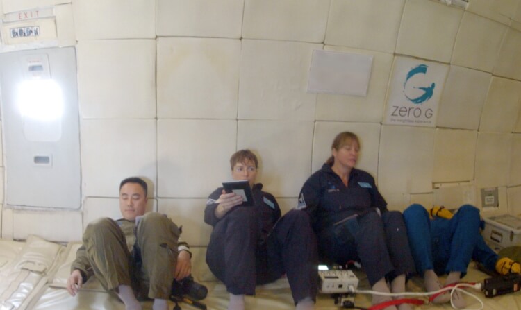
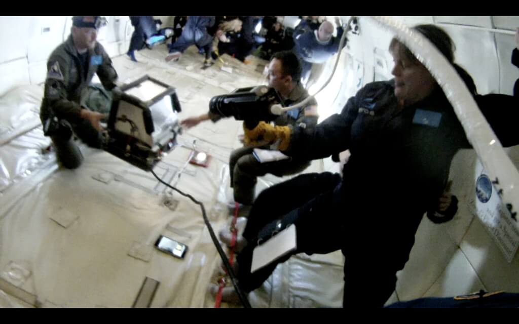
“That was short. That was very short.” My comments after the very first parabola, which was a Martian (0.33 G) scenario. This image shows our team’s positions in between parabola 1 & 2. We did not have space enough to fully lay down so we reclined against the side of the aircraft. Left to right is Con Tsang, myself (monitoring a payload via a table), Cathy Olkin, and Alan Stern (face not visible). The photo is taken via Go-Pro camera on the head of Dan Durda who was across the way. Eric Schindhelm, who rounded out our team, was next to Dan and not in this view.

The rapid change between the onset of low-gravity for about 10-15 seconds followed by 2-3 sec transition to what appeared to be about 30s of 1.8-2G forces was very unexpected. With each parabola I did start to realize that the set-up time for the manual operation of one payload took way too long. (Lesson learned)

Sometimes we had unexpected escapes (I escaped my foot-holds on Parabola #7) and Eric Schindhelm (shown below) escaped the next one.

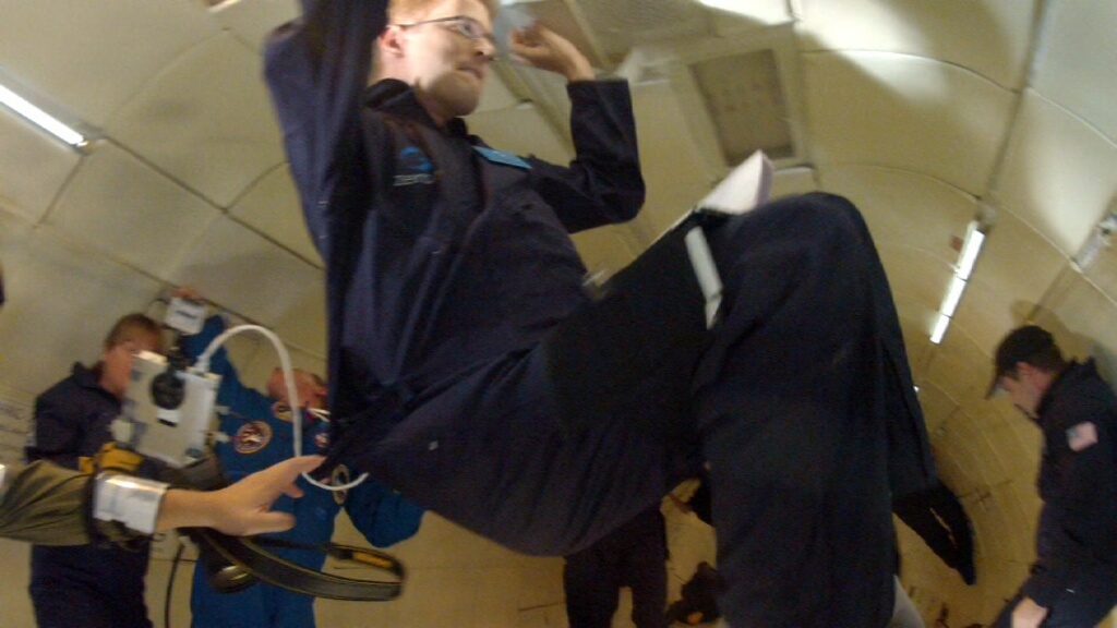
Con was monitoring BORE and deftly diverted Eric’s collision path. For BORE, the key thing was to keep the box free from any jostling by others or the cables.

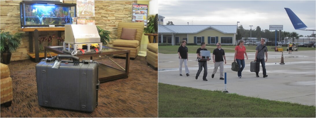
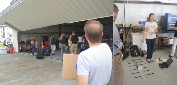
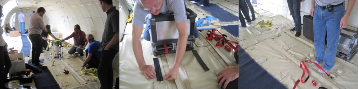
The payloads. We had two payloads, each with different goals for the flight. The fact that a decision to tether them together (made a few weeks before the flight) complicated the conops (concept of operations). One was a true science experiment: BORE, the Box of Rocks Experiment. The other was primarily an operations test for the SWUIS, the Southwest Universal Imaging System. Both experiments are pathfinder experiments for the emerging class of reusable commercial suborbital vehicles. Providers like Virgin Galactic, X-COR, Masten Space Systems, Up Aerospace, Whittinghill Aerospace, etc. You can read more about this fleet of exciting platform at NASA’s Flight Opportunity page https://flightopportunities.nasa.gov/, where they have links to all the providers.

From left to right: Dan & Con monitoring BORE (aluminum box with foamed edges) while Cathy holds onto the SWUIS camera doing a “human factors” test using a glove (yellow). Image from Go-Pro camera affixed to the SWUIS control box.

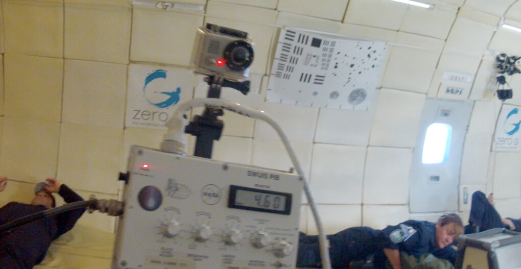
View of the SWUIS control box and Go-pro camera (used for situation awareness) while Dan’s holding it. You can see the SWUIS target that we used for the operations testing.  Image from a Go-Pro camera affixed to Dan’s head. Multiple cameras for context recording were definitely a must! (Lesson Learned)

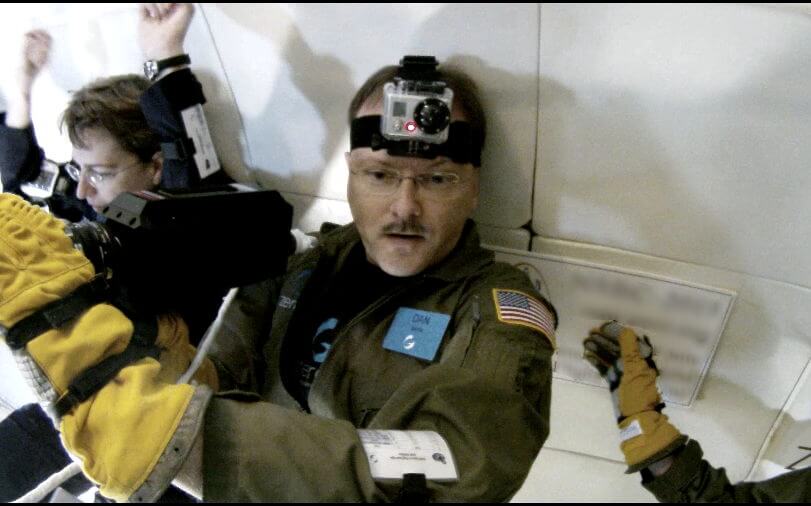
Dan Durda taking a test run with SWUIS on Parabola #23 (19^th zero-G).

With BORE, we ask the question: how do macro-sized particles interact in zero gravity? When you remove “gravity” from the equation, other forces (like electro-static, Van der Waals, capillary, etc.) dominate. In a nut shell, BORE is a simple experiment to examine the settling effects of regolith, the layer of loose, heterogeneous material covering rock, on small asteroids.

Our goal is to measure the effective coefficient of restitution (http://en.wikipedia.org/wiki/Coefficient_of_restitution) in inter-particle collisions while in zero-g conditions. The experiment consists of a box of rocks. There are two boxes, one filled with rocks of known size and density, one filled with random rocks. Video imagery (30fps) is taken of the contents of each box during the flight. After the flight, the plan is to use different software (ImageJ, Photoshop, and SynthEyes) to analyze the rocks and track their movements from frame to frame. The cost of BORE is less than $1K in total, making it in reach of a the proceeds of a High School bake sale!

BORE does need more than 20 s of microgravity to enable a better assessment of rock movement, and this is exactly why this experiment is planned for a suborbital flight where 4-5 minutes of microgravity conditions can be achieved. Here, we used the parabolic flight campaign to test the instrumentation and get a glimpse of the first few seconds of the rock behavior. With this series of 15-20s of microgravity, we made leaps forward from previous tests using drop towers which provide only 1-2s of microgravity.

Today’s Microgravity platforms and durations of zero-G fromhttp://www.nasa.gov/audience/foreducators/microgravity/home/.

• Drop Towers (1-5 s)
• Reduced-Gravity Aircraft (10-20s)
• Sounding Rockets (several minutes)
• Orbiting Laboratories such as the International Space Station (days)

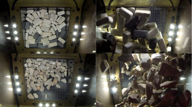
Some BORE images from one of the zero-G parabolas. Top Row: (left) Rest position of and (right) free-floating bricks of known size (they are actually bathroom tiles from Home Depot) but have the ratio L:W:H of 1.0:0.7:0.5. Surprisingly this is near the size and ratio of fragments created from laboratory impact experiments (e.g. Capaccioni, F. et al. 1984 & 1986, Fujikawa, A. et al. 1978) and similar to the ratio of shapes of boulders discovered on the rubble-pile asteroid Itokawa (see below).

Why is this important? Well, if you want to visit an asteroid someday and are designing tools to latch onto it, drill/dig into it, collect samples, etc. the behavior of collisional particles in this micro/zero-gravity environment is important. Scientifically, if you want to understand more about the formation, history and evolution of an asteroid where collisional events are significant, knowing more about how bombardment and repeated fragmentation events work is a key aspect.

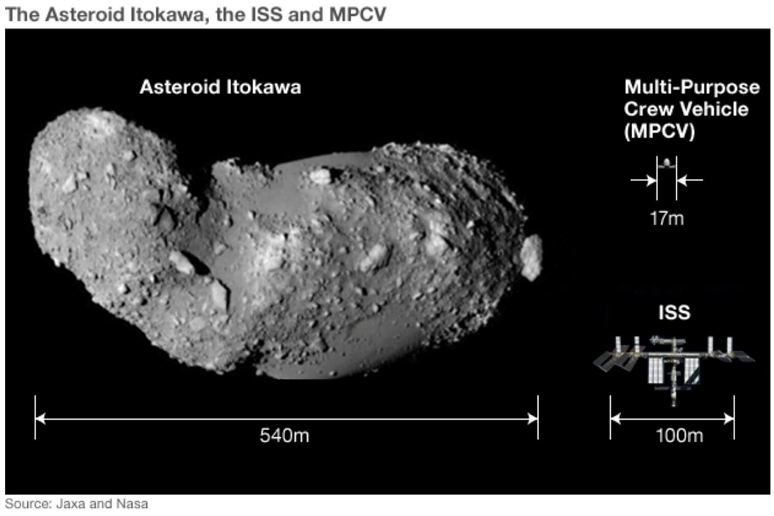
Source: NASA & JAXA. The first unambiguously identified rubble pile. Asteroid 25143 Itokawa observed by JAXA’S Hayabusa spacecraft. (Fujiwara, A. et al. 2006). The BORE experiment explored some of the settling processes that would have played a role in this object’s formation.

SWUIS was more of a “operations experiment.” This camera system has been flown on aircraft  before to hunt down elusive observations that require observing from a specific location on earth. For example, to observe an occultation event, when a object (asteroid, planet, moon) in our solar system crosses in front of a distant star, the projected “path” of the occultation on our planet is derived from the geometry and time of the observation, similar to how the more familiar solar and lunar eclipses only are visible from certain parts of the Earth at certain times. Having a high-performance astronomical camera system on a flying platform that can go to where you need to observe is powerful. So, SWUIS got its start in the 1990s when it was used on a series of aircraft. You can read more about those earlier campaigns at http://www.boulder.swri.edu/swuis/swuis.instr.html.

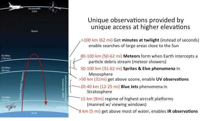
Over the past few years I have been helping a team at the Southwest Research Institute update this instrument for use on suborbital vehicles that get higher above the earth’s atmosphere compared to conventional aircraft. Suborbital vehicles can get to 100 km (328,000 ft.; 62 miles) altitude, whereas aircraft fly mainly at 9-12 km (30,000-40,000 ft.; 5.6-7.5 miles). Flying higher provides a unique observational space, both spectrally (great for infrared and UV as you are above all of the water and ozone, respectively), temporarily (you can look along the earth’s limb longer before an object “sets” below the horizon) and from a new vantage point (you can look down on particle debris streams created by meteors or observe sprites & elves phenomena in the mesosphere). 100km altitude is still pretty low compared to where orbiting spacecraft live, which is 160-2000 km (99-1200 miles) up (LEO/Low Earth Orbit). For example, our orbiting laboratory, the International Space Station is 400 km (250 miles) in altitude.

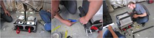
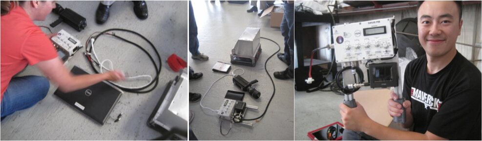
The SWUIS system today consists of a camera and lens, connected by one cable to a interface box. The interface box, which is from the 1990s version, allows one to manually control gain and black-level adjustments via knobs. It also provides a viewfinder in the form of a compact LCD screen. Data is analog but then digitized to a frame-grabber housed in a laptop. The 1990s version had a VCR to record the data, but since we are in the digital age, the battery-operated laptop augmentation was a natural and easy upgrade. The camera electronics are powered by a battery which makes it portable and compact. For this microgravity flight I introduced the notion of a tablet to control the laptop, to allow for the laptop to be stowed away. In practice this worked better than expected and my main take away is that the tablet is best fixed to something rather than hand-held to prevent unwanted “app-closure.” However, having a remote terminal for the laptop also would work.

Here’s a series of three short videos (no sound) of three legs when I got to hold the Xybion camera on Parabolas #13, 14 & 15. This captures how terribly short all the parabolas are and if you are doing an operations experiment, how utterly important it is to be positioned correctly at the start. One test was to position myself and get control of the camera and focus on a test target. A second test was to practice aiming at one target and then reposition for another target within the same parabola.

SWUIS_ZeroG_Parabola13_Web2

SWUIS_ZeroG_Parabola14_Web2

SWUIS_ZeroG_Parabola15_Web2

Above, the links are for lo-res (to fit within the upload file size restrictions on this site), no sound Videos of Parabola #13,14,15  (7,8 &9^th in microgravity). By the third time I was getting faster at set-up and on-target time.

In 1-G this camera and lens weigh 6.5 lbs. (3 kg) . Held at arms length, when I was composing the test in my lab, as I scripted the steps, I had trouble controlling the camera. In fact, I was shaking to keep camera on target after some seconds. I was amazed at how easy it was to hold this in zero-G, and complete the task. The Zero-G flight told us many things we need to redesign. One issue we learned was the tethering cabling was not a good idea and in some cases the camera, held by one person, was jerked from the control box, held by another person. In the next iteration, one of those items will need to be affixed to a structure to remove this weakness.

My lessons learned from the whole experience: Everything went by very quickly. Being tethered was difficult to maintain. Design the conops differently (what we did seemed awkward). Laptop and tablet worked better than expected. Hard to concentrate on something other than the task at hand. Don’t plan too much. Have multiple cameras viewing the experiment. Need to inspect the cable motion via video, as it was hard to view it in-situ. Very loud, hard to heard, hard to know what other people were working on. The video playback caught a lot more whoops during transitions to zero-G than I remembered. Heard the feet-down call clearly but not the onset of zero-G. The timing between parabolas is very short. The level breaks were good to reassemble the cabling then. Next time, don’t hang onto the steady-wire which is attached to the plane (I got that idea from Cathy & Alan next to me) as it caused more motion than needed (the plane kept moving into me): instead remain fixed with the footholds and do crouch positions like Con & Dan did and let the body relax (Con & Dan were most elegant).

And, my biggest take-away of all: If you want to do a microgravity experiment, I strongly recommend doing a “reconnaissance” flight first. Request to tag along a research flight to observe, perhaps lend a hand as some research teams might need another person. Observe the timing and cadence and space limitations. Use that to best perform your experiment. It is an amazing platform for research and engineering development and can truly explore unique physics and provide a place to explore your gizmo’s behavior in zero-G and find ways to make it robust before taking it to the launch pad.

I am very much hoping to experience microgravity again! With these same two payloads or with others. One of the key points of these reduced-gravity flights, they fly multiple times a year, so in theory, experiment turn-around is short. Ideally I wished we flew the next day. I could have implemented many changes in the payload-operations and also in Kimberly-operations.

Our team is now working to assess what worked and what did not work on this flight. We achieved our baseline goals, so that is great! Personally, I wished I had not been that focused on certain aspects of the payload performance and made more time to look around. However, that said, my focus keyed me on the task at hand, the payload performed better than expected, and when you have 10-15s, focus is the name of the game!

Reposted from https://blogs.nasa.gov/mission-ames/2013/12/17/its-time-to-fly-and-go-weightless-microgravity-flight-day-nov-17-2013-part-1-tsa-check-board-ascent-and-flight-profile/.

Reposted from https://blogs.nasa.gov/mission-ames/2013/12/16/this-little-scientists-first-taste-of-microgravity-research-aboard-a-reduced-gravity-aircraft-flight-day-minus-1-nov-16-2013-briefing-test-readiness-review-trr-and-load-up-the-plane/.

This is the first of a three-blog series (part 2 here, part 3 here) of this little scientist’s first foray into microgravity research. I participated in a research flight provided by the Zero-G corporation. To read more about their company go to https://www.gozerog.com/.

Zero-G operates a Boeing 727-200F aircraft, “G-Force One,” specially modified for reduced gravity operations. They provide opportunities for research flights (people and equipment) and also opportunities for you to experience zero-G (people). For experiment/research flights, you can apply directly to Zero-G where they organize a flight once they have enough researchers to fill a flight, or apply to NASA through their Flight Opportunities program https://flightopportunities.nasa.gov/, when NASA organizes the flight-manifest and Zero-G provides the flight platform. University students have additional opportunities to get flights through NASA’s Microgravity University,http://microgravityuniversity.jsc.nasa.gov/, with annual proposal calls. Had I known this when I was at school, I totally would have been a veteran flyer by now! Aircraft doing parabolic flight profiles are not restricted to the USA or to NASA. One list is provided here http://en.wikipedia.org/wiki/Reduced_gravity_aircraft.

The day before the flight, the flight director and series of “coaches” provided by the Zero G Corporation, came around to each of the research groups to look at the payloads and ascertain safety items. Prior to our arriving at our departure airport (in our case, Titusville, FL, but the “G-Force One” does fly from many airports, see their website), each team had to complete a Research Package, which contains the usual information such as mass, volume, power (including specifying “kill switch” items) and particular requests for gravity (the pilots can fly the airplane to simulate Martian and Lunar gravity in addition to near zero-G).  A series of weekly telecons were held in the weeks leading up to the flight to discuss interface needs and potential interference issues with others sharing the flight.

We meet the other teams for the first time. There were 6 experiments aboard this flight along with a BBC crew for the show Stargazing Live. One of the BBC presenters, Dara Ó Briain, joined us on this flight. So Kimberly gets to be an (unnamed) extra on TV show!

The other research experiments included (1) CubeSat solar-sail deployment mechanism, (2) testing a new IMU (inertia measurement unit), (3) evaluating sedimentations under Martian gravity, (4) Australian company developing ways to brew, and pour beer in zero-gravity, and (5) a mystery payload as it was under a NDA (non-disclosure agreement) with Zero G. Our Box of Rock science experiment (BORE) plus the SWUIS (Southwest Universal Imaging System) operations experiment rounded us to a total of 7 unique experiments. It was very fun getting to know the other experimenters, many who were also first timers!

(left) Our two payloads in the hotel before driving out to the airport. (right) Easy to transport our suitcase-sized payloads to the airfield.

(left) Heading to the Test Readiness Review (TRR). Payloads coming in cardboard boxes, pelican cases and roller bags. (right) Julia Laystrom-Woodard, a senior engineer from CU Aerospace (another first time flyer like me) describing her solar sail deployment experiment at the TRR.

The Test Readiness Review (TRR) was held in a hangar near the plane. Each group had to show the Zero-G staff the exact payload and configuration and describe the experiment in more detail and call attention to unique configurations and requests. In our case, we were going to use both blue tooth and wireless communication to monitor our payloads during the flight, so this meant an interference test with the airplane would need to be scheduled later in the day. The reviewers were mainly concerned about safety, safety to ourselves, safety to fellow passengers and equipment nearby, and safety to the airplane. For example, we had filed down edges on our payload, but due to the free-floating nature of the experiment, they requested we “foam our edges.” As we had experienced flyers with us, we had brought foam pipe-insulation with us and, of course, the ever-essential duct tape.  However, we had to send a few members of our team over lunch to Home Depot to pick up some more. Duct tape and foam were the order of the day!

Assembling BORE for the TRR. No shortage of duct tape and foam.

Assembling SWUIS and showing the layout of the tethering cables.

After the TRR, we waited for our time to set up in the aircraft. Along the floor of the aircraft are designated hook points. All payloads need to be secured to the floor with straps. For those that are “free-floating” they need to be secured within a storage box, whose dimensions were given to use prior. In our case, we configured our two free floating payloads to the size of two suitcase volumes. With our team of six, we identified where wanted our “footholds” to help keep us in place. These footholds were manually installed by the Zero-G folks and torqued down.

Loading up the plane via the back door to this Boeing 727. Not shown is that is another way to enter the aircraft via a large cargo bay door that can be opened on the side of the fuselage for larger payloads. For this flight, all the researcher’s experiments were all hand carried and broken down into smaller suitcase sized parts.

(left) Securing one of the other experiments to the floor of the aircraft. You can see the large cargo door opened to the left. It was a hot day in Titusville, FL so it made setting up a bit cooler to have air circulating. (middle) Using loads of Velcro to provide “temporary” binding for our free-floating experiments during the high-G times. (right) Setting up and installing the foot straps (red cords) to specific locations on the  floor.

During this setup we learned where each group would be physically situated on board and we could re-assess interference items not previously considered. Each experimenter group was assigned a 10 foot x10 foot area on the plane and were designated by the color of their socks. We were the “grey team” and had a spot about half-way down the aircraft near the exit windows.

After the configuration of all the mechanical hold-down areas, we did our powered tests and also checked for interference. All looked good. Anything we would bring the next day to board the flight had to fit in our flight suit. We next stowed our two suitcase payloads for takeoff and headed back to the hotel for a team briefing and light dinner.

The next blog entries follow the flight day.